Session 8: Reshaping Your Data
Using pivot functions from the tidyverse to change the shape of your data.
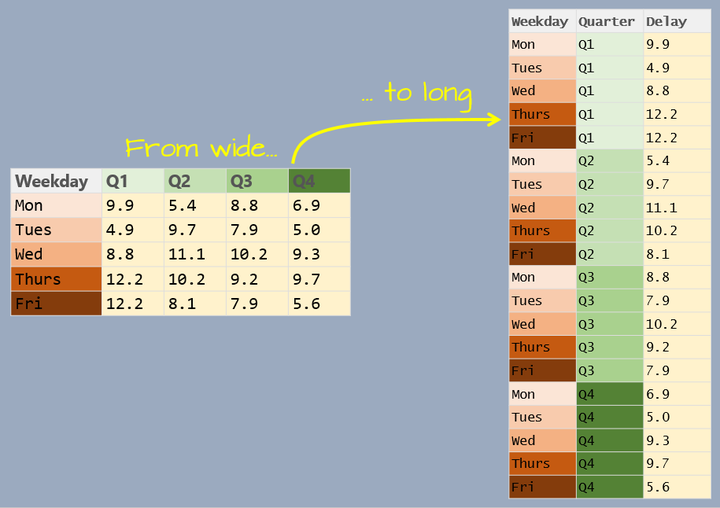 Image by Manny Gimond http://mgimond.github.io/
Session Goals
- Describe differences in long data vs wide data.
- Identify scenarios where it might be helpful to have data in one format over another (longer vs. wider).
- Use the functions
pivot_longer()andpivot_wider()to reshape data. - Use NHANES data to address whether blood pressure values vary in a predictable way with successive measurements.
Intro: The Shape Of A Dataset
A single set of data can sometimes be stored in different ways, or in other words, it can have different shapes. Below is a small example. It’s a hypothetical dataset that stores the number of visitors at each of two parks over a long weekend, and we’ll look at two different versions of it…
Wide Format
#create the dataset
visitors_wide <- data.frame("park" = c("north_park", "south_park"),
                   "Fri" = c(65, 80),
                   "Sat" = c(184, 160),
                   "Sun" = c(135, 140),
                   "Mon" = c(87, 71))

#view the dataset
visitors_wide

#>         park Fri Sat Sun Mon
#> 1 north_park  65 184 135  87
#> 2 south_park  80 160 140  71
Long Format
#create the dataset
visitors_long <- data.frame("park" = rep(c("north_park", "south_park"), 4),
                   "day" = c("Fri","Fri","Sat","Sat","Sun","Sun","Mon","Mon"),
                   "visitors" = c(65,80,184,160,135,140,87,71))

#view the dataset
visitors_long

#>         park day visitors
#> 1 north_park Fri       65
#> 2 south_park Fri       80
#> 3 north_park Sat      184
#> 4 south_park Sat      160
#> 5 north_park Sun      135
#> 6 south_park Sun      140
#> 7 north_park Mon       87
#> 8 south_park Mon       71
Notice that both datasets store the same information - it’s just formatted differently. These two datasets can be said to have different shapes. The first has a wider shape - it has more columns, stretching it out from left to right. The second has a longer shape, as it has fewer columns and more rows. Again, importantly, both datasets store the same information.
What Shape Should Your Data Be In?
The best answer to the question of what shape your data should be in is probably something like ‘Whatever shape makes it easiest to accomplish your goals with the data at any given time’. For example, sometimes when you’re entering data - say in to a spreadsheet in Excel or a similar program, you might find the data entry process easier if the dataset is in a wider format. In contrast, longer formats will generally be better when analyzing your data. This is consistent with the idea of tidy data we talked about in Session 2. For example, tidy data will be long because a characteristic of tidy data is that each variable has its own column. For these reasons, you might find it helpful or even necessary to reshape the data - possibly multiple times as you continue to work with the same dataset.
How To Reshape Data
R offers several approaches for reshaping data. Functions for doing so often come in pairs that transform from wider to longer, and longer to wider, respectively. Pairs of functions include cast() and melt(), spread() and gather(), and pivot_longer() and pivot_wider(). While any of these can be used, we’ll focus on the ‘pivot’ pair that come from the package tidyr, as they were written most recently with a goal of being the most user-friendly of the available functions so far.
Pivoting Resources
If you want to dig in to pivoting a bit more, R offers a very useful vignette on pivoting, which is worth a look - portions of today’s breakout sessions will come from there. Chapter 12 of “R For Data Science” by Wickham and Grolemund, which covers tidy data, also includes a nice section on pivoting.
Examples
Let’s revisit the park visitors dataset for an example of how pivot_longer() and pivot_wider() work in their most basic form. Previously, I created each of the wide and long forms of this dataset by hand. It was manageable to do that, since it’s a very small dataset, but for most datasets, you’re not going to want to just recreate a data frame from scratch each time you need to reshape the data. Let’s start with the data in wide format…
#view the data frame
visitors_wide

#>         park Fri Sat Sun Mon
#> 1 north_park  65 184 135  87
#> 2 south_park  80 160 140  71
What if we wanted to plot the total mean number of visitors per day across both parks? To get the mean values, we might think about applying some of the functions we’ve been working with in previous sessions like group_by() and summarize(). For example, we might want to try grouping by day and then calculating the means from a column that stores the number of visitors. However, in it’s current wide form, this dataset doesn’t have the day and visitors columns we need. pivot_longer() can help us here. The command might look like this…
library(tidyverse)
visitors_longer <- visitors_wide %>%
                   pivot_longer(-park,
                                names_to = "day",
                                values_to = "visitors")
First, we need to point it to the dataset we’re interested in reshaping - I’m doing that by piping the visitors_wide data frame to pivot_longer(). Next, we need to specify what columns to use to lengthen the dataset. This argument recognizes tidy-select notation, which can really simplify things. Here, I’m using -park, which tells it to use all the column names except park. Those column names will be transformed to values in a single new column, which needs a name. We’ll call it day, so names_to = "day". Finally, the values in the current columns will be stacked in to a single column, and it too needs a name, so values_to = "visitors". This lengthens the dataset, taking it from 5 columns down to 3.
#view the data
visitors_longer

#> # A tibble: 8 x 3
#>   park       day   visitors
#>   <fct>      <chr>    <dbl>
#> 1 north_park Fri         65
#> 2 north_park Sat        184
#> 3 north_park Sun        135
#> 4 north_park Mon         87
#> 5 south_park Fri         80
#> 6 south_park Sat        160
#> 7 south_park Sun        140
#> 8 south_park Mon         71
In this longer format, we’re able to apply the group_by() and summarize() functions…
visitors_longer %>%
    group_by(day) %>%
    summarise("mean" = mean(visitors))

#> `summarise()` ungrouping output (override with `.groups` argument)

#> # A tibble: 4 x 2
#>   day    mean
#>   <chr> <dbl>
#> 1 Fri    72.5
#> 2 Mon    79
#> 3 Sat   172
#> 4 Sun   138.
And we can go in the opposite direction with pivot_wider()…
visitors_longer %>%
  pivot_wider(names_from = day,
              values_from = visitors)

#> # A tibble: 2 x 5
#>   park         Fri   Sat   Sun   Mon
#>   <fct>      <dbl> <dbl> <dbl> <dbl>
#> 1 north_park    65   184   135    87
#> 2 south_park    80   160   140    71
The examples above represent the most basic uses of pivot_longer() and pivot_wider(). But each of these functions offer additional arguments that can help deal with more complicated situations. The next example is from the pivoting vignette I referenced above. It uses the billboard dataset that should already be available in your R session, and that stores weekly rankings of Billboard top 100 songs from the year 2000.
#preview billboard data
head(billboard)

#> # A tibble: 6 x 79
#>   artist track date.entered   wk1   wk2   wk3   wk4   wk5   wk6   wk7   wk8
#>   <chr>  <chr> <date>       <dbl> <dbl> <dbl> <dbl> <dbl> <dbl> <dbl> <dbl>
#> 1 2 Pac  Baby… 2000-02-26      87    82    72    77    87    94    99    NA
#> 2 2Ge+h… The … 2000-09-02      91    87    92    NA    NA    NA    NA    NA
#> 3 3 Doo… Kryp… 2000-04-08      81    70    68    67    66    57    54    53
#> 4 3 Doo… Loser 2000-10-21      76    76    72    69    67    65    55    59
#> 5 504 B… Wobb… 2000-04-15      57    34    25    17    17    31    36    49
#> 6 98^0   Give… 2000-08-19      51    39    34    26    26    19     2     2
#> # … with 68 more variables: wk9 <dbl>, wk10 <dbl>, wk11 <dbl>, wk12 <dbl>,
#> #   wk13 <dbl>, wk14 <dbl>, wk15 <dbl>, wk16 <dbl>, wk17 <dbl>, wk18 <dbl>,
#> #   wk19 <dbl>, wk20 <dbl>, wk21 <dbl>, wk22 <dbl>, wk23 <dbl>, wk24 <dbl>,
#> #   wk25 <dbl>, wk26 <dbl>, wk27 <dbl>, wk28 <dbl>, wk29 <dbl>, wk30 <dbl>,
#> #   wk31 <dbl>, wk32 <dbl>, wk33 <dbl>, wk34 <dbl>, wk35 <dbl>, wk36 <dbl>,
#> #   wk37 <dbl>, wk38 <dbl>, wk39 <dbl>, wk40 <dbl>, wk41 <dbl>, wk42 <dbl>,
#> #   wk43 <dbl>, wk44 <dbl>, wk45 <dbl>, wk46 <dbl>, wk47 <dbl>, wk48 <dbl>,
#> #   wk49 <dbl>, wk50 <dbl>, wk51 <dbl>, wk52 <dbl>, wk53 <dbl>, wk54 <dbl>,
#> #   wk55 <dbl>, wk56 <dbl>, wk57 <dbl>, wk58 <dbl>, wk59 <dbl>, wk60 <dbl>,
#> #   wk61 <dbl>, wk62 <dbl>, wk63 <dbl>, wk64 <dbl>, wk65 <dbl>, wk66 <lgl>,
#> #   wk67 <lgl>, wk68 <lgl>, wk69 <lgl>, wk70 <lgl>, wk71 <lgl>, wk72 <lgl>,
#> #   wk73 <lgl>, wk74 <lgl>, wk75 <lgl>, wk76 <lgl>
Notice there are columns named ‘wk1’ through ‘wk73’ that store the weekly ranking for each song. Week itself is a variable with values that could be represented in a single column. We could do something similar to our above use of pivot_longer()…
billboard %>%
  pivot_longer(cols = starts_with("wk"),
               names_to = "week",
               values_to = "rank") %>%
  head()

#> # A tibble: 6 x 5
#>   artist track                   date.entered week   rank
#>   <chr>  <chr>                   <date>       <chr> <dbl>
#> 1 2 Pac  Baby Don't Cry (Keep... 2000-02-26   wk1      87
#> 2 2 Pac  Baby Don't Cry (Keep... 2000-02-26   wk2      82
#> 3 2 Pac  Baby Don't Cry (Keep... 2000-02-26   wk3      72
#> 4 2 Pac  Baby Don't Cry (Keep... 2000-02-26   wk4      77
#> 5 2 Pac  Baby Don't Cry (Keep... 2000-02-26   wk5      87
#> 6 2 Pac  Baby Don't Cry (Keep... 2000-02-26   wk6      94
This is a start - we’ve gone from 79 columns to just 6. But we can clean this up a bit more. Notice the values in the new week column all include the ‘wk’ prefix. Since we’ve labeled the column ‘week’, it’s kind of redundant and unnecessary to have ‘wk’ at the beginning of each value. We can add the ‘names_prefix’ argument, which accepts a regular expression (regex). Characters at the beginning of column names that match the regex get removed.
billboard %>%
  pivot_longer(cols = starts_with("wk"),
              names_to = "week",
              values_to = "rank",
              names_prefix = "wk") %>%
  head()

#> # A tibble: 6 x 5
#>   artist track                   date.entered week   rank
#>   <chr>  <chr>                   <date>       <chr> <dbl>
#> 1 2 Pac  Baby Don't Cry (Keep... 2000-02-26   1        87
#> 2 2 Pac  Baby Don't Cry (Keep... 2000-02-26   2        82
#> 3 2 Pac  Baby Don't Cry (Keep... 2000-02-26   3        72
#> 4 2 Pac  Baby Don't Cry (Keep... 2000-02-26   4        77
#> 5 2 Pac  Baby Don't Cry (Keep... 2000-02-26   5        87
#> 6 2 Pac  Baby Don't Cry (Keep... 2000-02-26   6        94
We haven’t dealt with regular expressions in Code Club yet - they’ll make a good topic for a future session, but if you’re interested in the meantime, I did a couple short videos introducing them as part of this set of videos on command line computing.
Breakout Rooms
In the breakout rooms, we’ll use a pivot function to analyze a portion of the NHANES dataset. We’ll use the data to try to address whether successive blood pressure measurements from the same individual differ in a predictable way.
If you haven’t already done it, you can install the NHANES dataset with…
install.packages("NHANES", repos = "http://cran.us.r-project.org")

#>
#> The downloaded binary packages are in
#>   /var/folders/s7/y_mgh3c54h9fjcyw9wqdkb8x4zs_jy/T//RtmpWxvWIv/downloaded_packages
Exercise 1
First let’s load and preview the NHANES dataset.
Hints (click here)
Use library() to load the dataset. The functions head() are glimpse() are a couple good options for previewing the data.
Solution (click here)
library(NHANES)
glimpse(NHANES)

#> Rows: 10,000
#> Columns: 76
#> $ ID               <int> 51624, 51624, 51624, 51625, 51630, 51638, 51646, 516…
#> $ SurveyYr         <fct> 2009_10, 2009_10, 2009_10, 2009_10, 2009_10, 2009_10…
#> $ Gender           <fct> male, male, male, male, female, male, male, female, …
#> $ Age              <int> 34, 34, 34, 4, 49, 9, 8, 45, 45, 45, 66, 58, 54, 10,…
#> $ AgeDecade        <fct>  30-39,  30-39,  30-39,  0-9,  40-49,  0-9,  0-9,  4…
#> $ AgeMonths        <int> 409, 409, 409, 49, 596, 115, 101, 541, 541, 541, 795…
#> $ Race1            <fct> White, White, White, Other, White, White, White, Whi…
#> $ Race3            <fct> NA, NA, NA, NA, NA, NA, NA, NA, NA, NA, NA, NA, NA, …
#> $ Education        <fct> High School, High School, High School, NA, Some Coll…
#> $ MaritalStatus    <fct> Married, Married, Married, NA, LivePartner, NA, NA, …
#> $ HHIncome         <fct> 25000-34999, 25000-34999, 25000-34999, 20000-24999, …
#> $ HHIncomeMid      <int> 30000, 30000, 30000, 22500, 40000, 87500, 60000, 875…
#> $ Poverty          <dbl> 1.36, 1.36, 1.36, 1.07, 1.91, 1.84, 2.33, 5.00, 5.00…
#> $ HomeRooms        <int> 6, 6, 6, 9, 5, 6, 7, 6, 6, 6, 5, 10, 6, 10, 10, 4, 3…
#> $ HomeOwn          <fct> Own, Own, Own, Own, Rent, Rent, Own, Own, Own, Own, …
#> $ Work             <fct> NotWorking, NotWorking, NotWorking, NA, NotWorking, …
#> $ Weight           <dbl> 87.4, 87.4, 87.4, 17.0, 86.7, 29.8, 35.2, 75.7, 75.7…
#> $ Length           <dbl> NA, NA, NA, NA, NA, NA, NA, NA, NA, NA, NA, NA, NA, …
#> $ HeadCirc         <dbl> NA, NA, NA, NA, NA, NA, NA, NA, NA, NA, NA, NA, NA, …
#> $ Height           <dbl> 164.7, 164.7, 164.7, 105.4, 168.4, 133.1, 130.6, 166…
#> $ BMI              <dbl> 32.22, 32.22, 32.22, 15.30, 30.57, 16.82, 20.64, 27.…
#> $ BMICatUnder20yrs <fct> NA, NA, NA, NA, NA, NA, NA, NA, NA, NA, NA, NA, NA, …
#> $ BMI_WHO          <fct> 30.0_plus, 30.0_plus, 30.0_plus, 12.0_18.5, 30.0_plu…
#> $ Pulse            <int> 70, 70, 70, NA, 86, 82, 72, 62, 62, 62, 60, 62, 76, …
#> $ BPSysAve         <int> 113, 113, 113, NA, 112, 86, 107, 118, 118, 118, 111,…
#> $ BPDiaAve         <int> 85, 85, 85, NA, 75, 47, 37, 64, 64, 64, 63, 74, 85, …
#> $ BPSys1           <int> 114, 114, 114, NA, 118, 84, 114, 106, 106, 106, 124,…
#> $ BPDia1           <int> 88, 88, 88, NA, 82, 50, 46, 62, 62, 62, 64, 76, 86, …
#> $ BPSys2           <int> 114, 114, 114, NA, 108, 84, 108, 118, 118, 118, 108,…
#> $ BPDia2           <int> 88, 88, 88, NA, 74, 50, 36, 68, 68, 68, 62, 72, 88, …
#> $ BPSys3           <int> 112, 112, 112, NA, 116, 88, 106, 118, 118, 118, 114,…
#> $ BPDia3           <int> 82, 82, 82, NA, 76, 44, 38, 60, 60, 60, 64, 76, 82, …
#> $ Testosterone     <dbl> NA, NA, NA, NA, NA, NA, NA, NA, NA, NA, NA, NA, NA, …
#> $ DirectChol       <dbl> 1.29, 1.29, 1.29, NA, 1.16, 1.34, 1.55, 2.12, 2.12, …
#> $ TotChol          <dbl> 3.49, 3.49, 3.49, NA, 6.70, 4.86, 4.09, 5.82, 5.82, …
#> $ UrineVol1        <int> 352, 352, 352, NA, 77, 123, 238, 106, 106, 106, 113,…
#> $ UrineFlow1       <dbl> NA, NA, NA, NA, 0.094, 1.538, 1.322, 1.116, 1.116, 1…
#> $ UrineVol2        <int> NA, NA, NA, NA, NA, NA, NA, NA, NA, NA, NA, NA, NA, …
#> $ UrineFlow2       <dbl> NA, NA, NA, NA, NA, NA, NA, NA, NA, NA, NA, NA, NA, …
#> $ Diabetes         <fct> No, No, No, No, No, No, No, No, No, No, No, No, No, …
#> $ DiabetesAge      <int> NA, NA, NA, NA, NA, NA, NA, NA, NA, NA, NA, NA, NA, …
#> $ HealthGen        <fct> Good, Good, Good, NA, Good, NA, NA, Vgood, Vgood, Vg…
#> $ DaysPhysHlthBad  <int> 0, 0, 0, NA, 0, NA, NA, 0, 0, 0, 10, 0, 4, NA, NA, 0…
#> $ DaysMentHlthBad  <int> 15, 15, 15, NA, 10, NA, NA, 3, 3, 3, 0, 0, 0, NA, NA…
#> $ LittleInterest   <fct> Most, Most, Most, NA, Several, NA, NA, None, None, N…
#> $ Depressed        <fct> Several, Several, Several, NA, Several, NA, NA, None…
#> $ nPregnancies     <int> NA, NA, NA, NA, 2, NA, NA, 1, 1, 1, NA, NA, NA, NA, …
#> $ nBabies          <int> NA, NA, NA, NA, 2, NA, NA, NA, NA, NA, NA, NA, NA, N…
#> $ Age1stBaby       <int> NA, NA, NA, NA, 27, NA, NA, NA, NA, NA, NA, NA, NA, …
#> $ SleepHrsNight    <int> 4, 4, 4, NA, 8, NA, NA, 8, 8, 8, 7, 5, 4, NA, 5, 7, …
#> $ SleepTrouble     <fct> Yes, Yes, Yes, NA, Yes, NA, NA, No, No, No, No, No, …
#> $ PhysActive       <fct> No, No, No, NA, No, NA, NA, Yes, Yes, Yes, Yes, Yes,…
#> $ PhysActiveDays   <int> NA, NA, NA, NA, NA, NA, NA, 5, 5, 5, 7, 5, 1, NA, 2,…
#> $ TVHrsDay         <fct> NA, NA, NA, NA, NA, NA, NA, NA, NA, NA, NA, NA, NA, …
#> $ CompHrsDay       <fct> NA, NA, NA, NA, NA, NA, NA, NA, NA, NA, NA, NA, NA, …
#> $ TVHrsDayChild    <int> NA, NA, NA, 4, NA, 5, 1, NA, NA, NA, NA, NA, NA, 4, …
#> $ CompHrsDayChild  <int> NA, NA, NA, 1, NA, 0, 6, NA, NA, NA, NA, NA, NA, 3, …
#> $ Alcohol12PlusYr  <fct> Yes, Yes, Yes, NA, Yes, NA, NA, Yes, Yes, Yes, Yes, …
#> $ AlcoholDay       <int> NA, NA, NA, NA, 2, NA, NA, 3, 3, 3, 1, 2, 6, NA, NA,…
#> $ AlcoholYear      <int> 0, 0, 0, NA, 20, NA, NA, 52, 52, 52, 100, 104, 364, …
#> $ SmokeNow         <fct> No, No, No, NA, Yes, NA, NA, NA, NA, NA, No, NA, NA,…
#> $ Smoke100         <fct> Yes, Yes, Yes, NA, Yes, NA, NA, No, No, No, Yes, No,…
#> $ Smoke100n        <fct> Smoker, Smoker, Smoker, NA, Smoker, NA, NA, Non-Smok…
#> $ SmokeAge         <int> 18, 18, 18, NA, 38, NA, NA, NA, NA, NA, 13, NA, NA, …
#> $ Marijuana        <fct> Yes, Yes, Yes, NA, Yes, NA, NA, Yes, Yes, Yes, NA, Y…
#> $ AgeFirstMarij    <int> 17, 17, 17, NA, 18, NA, NA, 13, 13, 13, NA, 19, 15, …
#> $ RegularMarij     <fct> No, No, No, NA, No, NA, NA, No, No, No, NA, Yes, Yes…
#> $ AgeRegMarij      <int> NA, NA, NA, NA, NA, NA, NA, NA, NA, NA, NA, 20, 15, …
#> $ HardDrugs        <fct> Yes, Yes, Yes, NA, Yes, NA, NA, No, No, No, No, Yes,…
#> $ SexEver          <fct> Yes, Yes, Yes, NA, Yes, NA, NA, Yes, Yes, Yes, Yes, …
#> $ SexAge           <int> 16, 16, 16, NA, 12, NA, NA, 13, 13, 13, 17, 22, 12, …
#> $ SexNumPartnLife  <int> 8, 8, 8, NA, 10, NA, NA, 20, 20, 20, 15, 7, 100, NA,…
#> $ SexNumPartYear   <int> 1, 1, 1, NA, 1, NA, NA, 0, 0, 0, NA, 1, 1, NA, NA, 1…
#> $ SameSex          <fct> No, No, No, NA, Yes, NA, NA, Yes, Yes, Yes, No, No, …
#> $ SexOrientation   <fct> Heterosexual, Heterosexual, Heterosexual, NA, Hetero…
#> $ PregnantNow      <fct> NA, NA, NA, NA, NA, NA, NA, NA, NA, NA, NA, NA, NA, …
Exercise 2
As you might know, blood pressure consists of two values - systolic and diastolic. Each participant in the NHANES survey had their blood pressure measured three times in succession, giving us the columns: BPSys1, BPDia1, BPSys2, BPDia2, BPSys3, BPDia3. Let’s work first with just the three systolic values.
Subset the dataset to get just the columns BPSys1, BPSys2, and BPSys3. Name the new object ‘sys_values’, then get the dimensions of sys_values and preview it.
Hints (click here)
Use select() from dplyr to get the three columns we want. dim() and glimpse() can be used to get the dimensions and preview the data, respectively.
Solution (click here)
sys_values <- NHANES %>%
    select(matches("BPSys[123]$"))
#I used the 'matches' helper along with a regular expression
#above, but there are a number of ways you could do this.
#One equivalent would be...
# sys_values <- NHANES %>% select(BPSys1, BPSys2, BPSys3)

dim(sys_values)

#> [1] 10000     3


head(sys_values)

#> # A tibble: 6 x 3
#>   BPSys1 BPSys2 BPSys3
#>    <int>  <int>  <int>
#> 1    114    114    112
#> 2    114    114    112
#> 3    114    114    112
#> 4     NA     NA     NA
#> 5    118    108    116
#> 6     84     84     88
Exercise 3
We can see just from the preview in Exercise 2 that the dataset has some missing data - let’s remove rows that have NA’s. Call the new dataset ‘sys_noNA’. Then check the dimensions and preview again.
Hints (click here)
Try the drop_na function from tidyr to eliminate rows containing missing data.
Exercise 4
We’ll explore these data a bit to see if there’s any evidence of a trend in systolic blood pressure with respect to the sequence of measurements (differences among measurements 1, 2, and 3). First, lets reshape the data so we end up with just two columns named ‘measurement’ and ‘sys_bp’. Save the new objects as ‘sys_long’. Then check the dimensions and preview again.
Hints (click here)
Use pivot_longer() to lengthen the dataset. You’ll need to include the arguments “cols”, “names_to”, and “values_to”.
Solution (click here)
sys_long <- sys_noNA %>%
  pivot_longer(cols = starts_with("BP"),
               names_to = "measurement",
               values_to = "sys_bp")

dim(sys_long)

#> [1] 23913     2


head(sys_long)

#> # A tibble: 6 x 2
#>   measurement sys_bp
#>   <chr>        <int>
#> 1 BPSys1         114
#> 2 BPSys2         114
#> 3 BPSys3         112
#> 4 BPSys1         114
#> 5 BPSys2         114
#> 6 BPSys3         112
Exercise 5
Now let’s calculate and compare the mean values for each measurement.
Hints (click here)
Use group_by() and summarize() to get a mean for each of the three measurements.
Solution (click here)
sys_long %>%
  group_by(measurement) %>%
  summarize("mean_sys" = mean(sys_bp))

#> `summarise()` ungrouping output (override with `.groups` argument)

#> # A tibble: 3 x 2
#>   measurement mean_sys
#>   <chr>          <dbl>
#> 1 BPSys1          119.
#> 2 BPSys2          118.
#> 3 BPSys3          118.
Exercise 6
The summarise() functions outputs a tibble. Tibbles are intended to be tidy, and as part of that, by default the values they display tend to be truncated/rounded to a greater degree than they would be otherwise in R. In this case, we might want to see a bit more precision in the values. Try adjusting (increasing) the number of significant figures that are displayed in the tibble that was output in Exercise 5.
Hints (click here)
This can be done in a couple different ways. One is to convert the tibble to a data frame with as.data.frame(), since data frames, by default, will likely show more significant digits. Alternatively, try setting options(pillar.sigfig) to a new value.
Solution (click here)
sys_long %>%
  group_by(measurement) %>%
  summarize("mean_sys" = mean(sys_bp)) %>%
  as.data.frame()

#> `summarise()` ungrouping output (override with `.groups` argument)

#>   measurement mean_sys
#> 1      BPSys1 119.1682
#> 2      BPSys2 118.4333
#> 3      BPSys3 117.8479


#OR

options(pillar.sigfig = 6)
sys_long %>%
  group_by(measurement) %>%
  summarize("mean_sys" = mean(sys_bp))

#> `summarise()` ungrouping output (override with `.groups` argument)

#> # A tibble: 3 x 2
#>   measurement mean_sys
#>   <chr>          <dbl>
#> 1 BPSys1       119.168
#> 2 BPSys2       118.433
#> 3 BPSys3       117.848
Bonus 1
Are those differences statistically significant? A one-way anova might be a good option to test that. Check out the help page for the function aov() and try running an ANOVA.
Hint 1 (click here)
R often uses the tilde (~) to indicate formula notation. So, for example, you can generate a scatterplot in base R by plotting y~x, assuming y and x are numeric vectors of equal lengths. The aov() function requires a formula with the pattern values~group. You can use the column names in the data frame to define these, but then you need to use the ‘data’ argument to tell the function the name of the data frame where those columns exist.
Bonus 2
Repeat all of the above for diastolic blood pressure with a couple of modifications along the way. First, when you reshape/lengthen the data, make the values in the ‘measurement’ column numeric. For example, in the sys_long data frame we created above, the values in the measurement column were characters, and looked like “BPsys1”. This time, make them a factor with the levels “1”, “2”, and “3”.
Hint (click here)
Use the pivot_longer() arguments “names_prefix” and “names_transform”.
Solution (click here)
dia_data <- NHANES %>%
  select(matches("BPDia[123]$")) %>%
  drop_na() %>%
  pivot_longer(cols = starts_with("BP"),
               names_to = "measurement",
               values_to = "dia_bp",
               names_prefix = "BPDia",
               names_transform = list(measurement = "as.factor"))

head(dia_data)

#> # A tibble: 6 x 2
#>   measurement dia_bp
#>   <fct>        <int>
#> 1 1               88
#> 2 2               88
#> 3 3               82
#> 4 1               88
#> 5 2               88
#> 6 3               82


dia_data %>%
  group_by(measurement) %>%
  summarize("mean_dia" = mean(dia_bp)) %>%
  as.data.frame()

#> `summarise()` ungrouping output (override with `.groups` argument)

#>   measurement mean_dia
#> 1           1 68.28830
#> 2           2 67.46280
#> 3           3 67.06762


aov(dia_bp~measurement, data = dia_data) %>%
  summary()

#>                Df  Sum Sq Mean Sq F value   Pr(>F)
#> measurement     2    6185  3092.3   14.91 3.38e-07 ***
#> Residuals   23910 4958916   207.4
#> ---
#> Signif. codes:  0 '***' 0.001 '**' 0.01 '*' 0.05 '.' 0.1 ' ' 1