Session 7: R Markdown
Text + Code + Output
 Artwork by @allison_horst
Introduction
R Markdown consists of an amazing ecosystem of R packages to produce many types of technical content. Its signature capability is that is can run R code and print the code along with its results and nicely formatted prose.
To understand R Markdown, we need to learn about three new things:
-
Markdown, a very lightweight text formatting language.
-
Code chunks, which allow us to incorporate R code that can be executed and whose results we can display in text, figures, and tables.
-
The YAML header, which encodes metadata about the output, such as the desired output format and specific formatting features.
We’ll focus on HTML page output, but will glimpse at the many possibilities for the output format: with R Markdown, it is possible to create not just technical reports, but also slide decks, websites, books, scientific articles, and so on.
Setup
At the core of the R Markdown ecosystem is the rmarkdown package. We need to install this but don’t need to load it:
install.packages("rmarkdown")
Inside your directory for Code Club, create a directory for this week:
dir.create('S07')
First, an example
Before we go into details, let’s first see a quick demonstration of what we are talking about:
-
Go to
File=>New File=>R Markdown, change the Title to “Markdown demo”, and clickOK. -
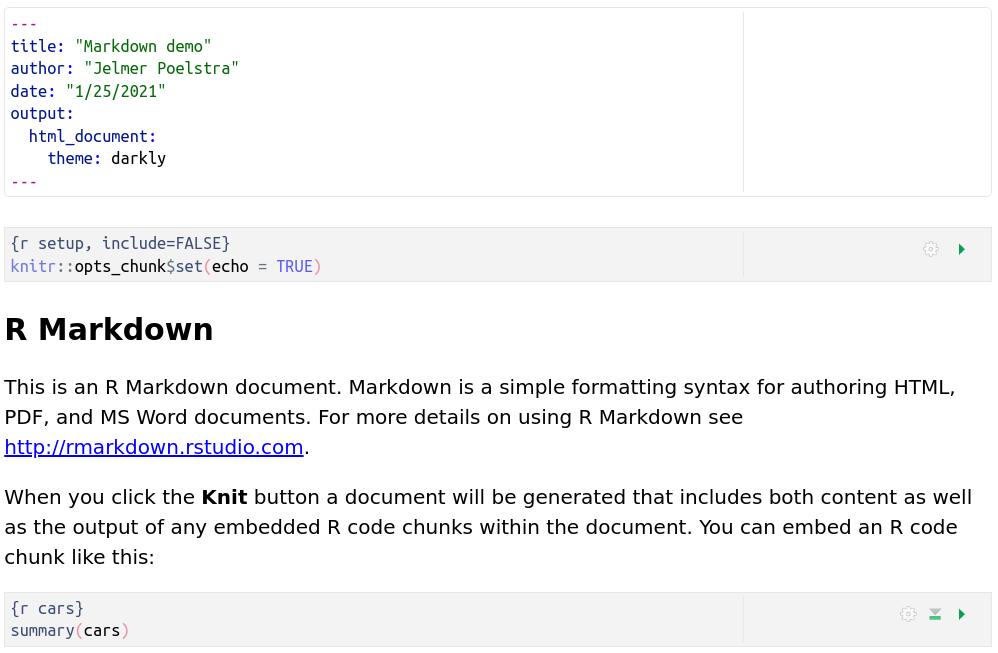
Take a look at the R Markdown document, and notice that there seems to be some sort of header (=> YAML), followed by R code wrapped in strange constructs with backticks (=> Code chunks), and plain written text (=> Markdown).
-
Before we can create output, we need to save the document. Click the
Savebutton and save the files asdemo.Rmdinside your newly created directory. -
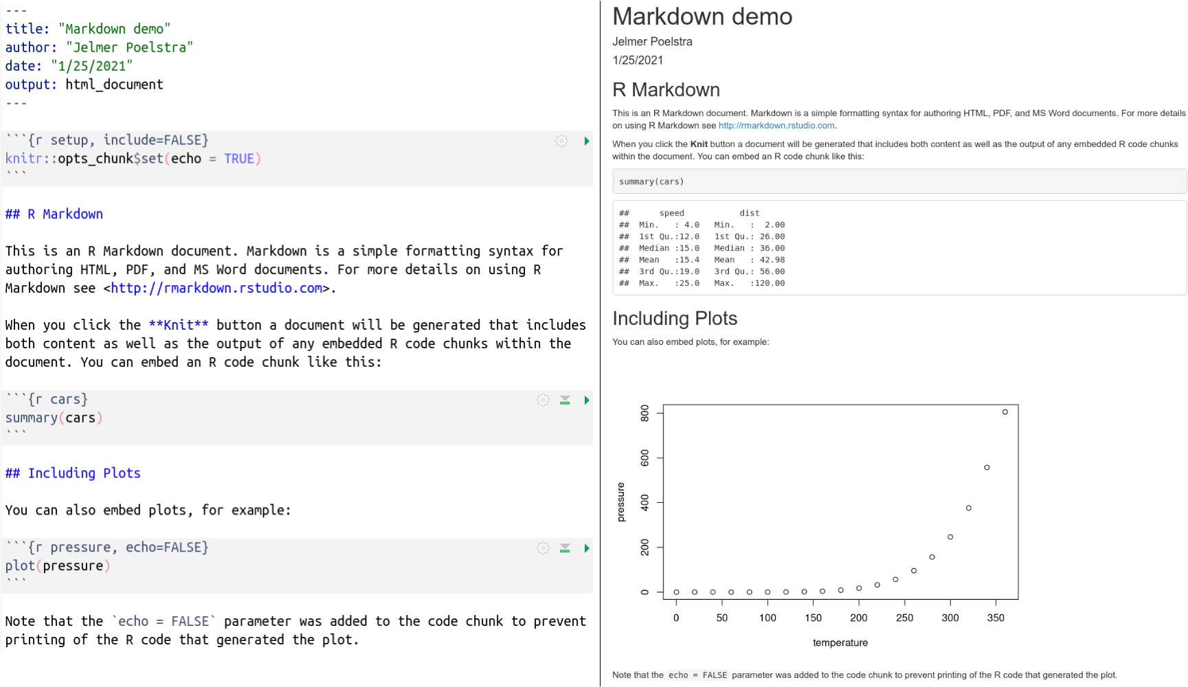
Now click the Knit button in one of the top bars, and a document should show up in a pop-up or the Viewer pane. This is the rendered output from the R Markdown document.
Notice that the YAML header is not printed, at least not verbatim, while some of the code is printed, and we also see code output including a plot!
This is what the raw and rendered output look side-by-side:
We’ll now talk about Markdown, code chunks, and the YAML header in turn.
I: Markdown
Markdown is a very lightweight language to format plain text files, which evolved from simple in-line formatting applied in emails before those started using HTML.
Need to emphasize a word without being able to make it italic or bold? How about adding emphasis with asterisks *like so*?
An overview of commonly used Markdown syntax
| Syntax | Result |
|---|---|
| # My Title | Header level 1 (largest) |
| ## My Section | Header level 2 |
| ### My Subsection | Header level 3 – and so forth |
| *italic* or _italic_ | italic |
| **bold** or __bold__ | bold |
[Markdown Guide](markdownguide.org) |
Markdown Guide (Link with custom text) |
|  | Figure |
| - List item | Unordered (bulleted) list |
| 1. List item | Ordered (numbered) list |
`inline code` |
inline code |
``` …code… ``` |
Generic code block (for formatting only) (Alternative syntax: 4 leading spaces.) |
```r …code… ``` |
r code block (for formatting only) |
--- |
Horizontal rule (line) |
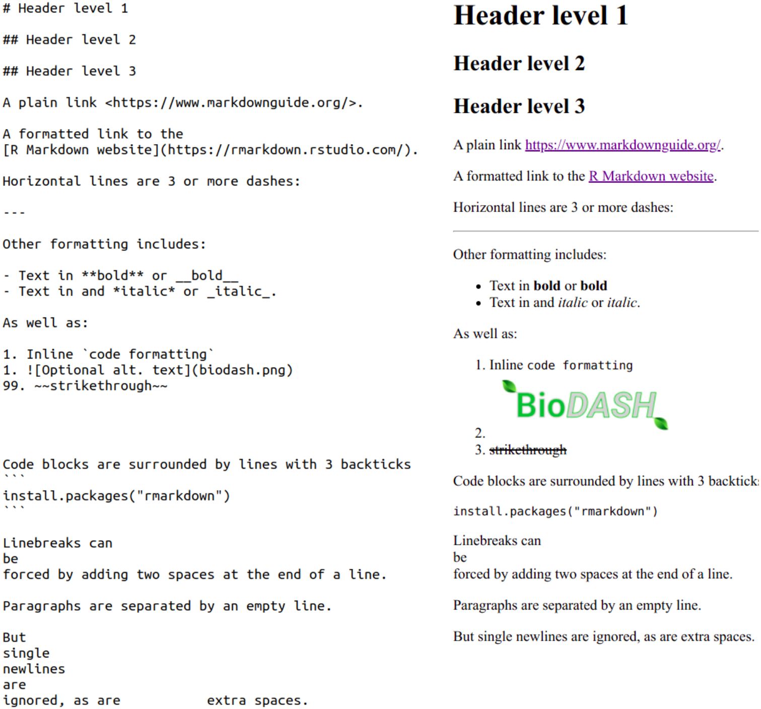
To see this formatting in action, see below an example of a raw Markdown file on the left, and its rendered (formatted) output on the right:
“Plain” Markdown files have the extension .md, whereas R Markdown files have the extension .Rmd.
II: Integrating R code
As we saw above, plain Markdown has syntax for code formatting, but the code is not actually being executed. In R Markdown, however, we are able run code! The syntax to do so is only slightly modified from what we saw above:
-
For inline code, we add
rand a space before the R code that is to be executed, for example:Raw Rendered There are `r 365*24`hours in a yearThere are 8760 hours in a year -
To generate code blocks, which we call code chunks in an R Markdown context,
we add r inside curly braces:```{r}We can optionally add settings that we want to apply to that chunk and/or chunk labels:
```{r, option1=value, ...}or```{r, unique-chunk-label, option1=value, ...}RStudio keyboard shortcut to insert a code chunk: Cmd/Ctrl+Alt+I.
Code chunk examples
-
A code chunk with default options…
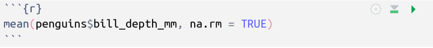
…will be executed and shown followed by the output of the code:
mean(penguins$bill_depth_mm, na.rm = TRUE) #> [1] 17.15117 -
As an example of using a code chunk option, we will disable printing the code using
echo=FALSE(the code will still run and the output will still be shown):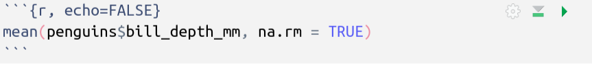
#> [1] 17.15117 -
Figures can, of course, also be printed:
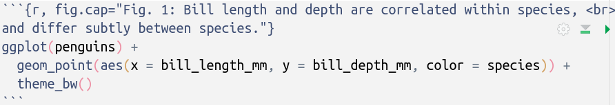
ggplot(penguins) +
  geom_point(aes(x = bill_length_mm, y = bill_depth_mm, color = species)) +
  theme_bw()

#> Warning: Removed 2 rows containing missing values (geom_point).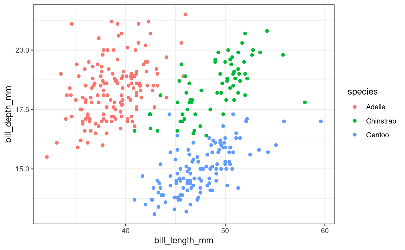
Fig. 1: Bill length and depth are correlated within species,
and differ subtly between species.
Above, we added a caption for the figure using the fig.cap argument (with a little trick to force a line break, using the <br> HTML syntax).
Code chunk options
Here is an overview of some the most commonly made changes to defaults for code chunk options. This quickly gets confusing, but you’ll get the hang of it after experimenting a bit.
echo=FALSE– Don’t print the code in the output file.eval=FALSE– Don’t run (evaluate) the code.include=FALSE– Run but don’t print the code, nor any of its results.results="hide"– Don’t print the text output of the code.fig.show="hide"– Don’t print figures produced by the code.
Furthermore, you can use message=FALSE and warning=FALSE to suppress any messages (like the output when loading packages) and warnings (like the warning for the penguin figure above), respectively, that R might produce.
For figures, the following options are especially useful:
fig.cap="My caption"– Include a caption.fig.asp=0.6– Aspect ratio.fig.width=6– Width of in inches: same as sizing in regular R code.fig.height=9.6– Height in inches: same as sizing in regular R code.out.width="70%"– Figure width as printed in the document (in%or pixels,px).out.height="500px"– Figure height as printed in the document.
Finally, if your document takes a long time to knit, use cache=TRUE to enable caching of results.
Default chunk options
It is often practical to set default chunk options for the entire document, and you can do so with the opts_chunk$set() function as shown below:
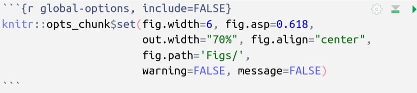
This is usually done in separate “global setup chunk” at the start of the document.
Whenever necessary, you can then override these defaults for specific chunks.
III: The YAML header
YAML (“YAML Ain’t Markup Language”) is a simple format commonly used for configuration files, which allows you to provide key-value pairs such as author: John Doe.
In R Markdown files, it is used as a header which configures certain aspects of the output, especially the formatting. Put another way, the YAML header contains the metadata for the output.
A basic YAML header
Here is an example of a very basic YAML header:
---
author: My name
title: The document's title
output: html_document
---
Note the lines which just contain three dashes, which mark the beginning and the end of the YAML header.
Adding options
Often, a value (like html_document) can itself be given key-value pairs to specify additional options – see the example below where we include a Table of Contents (toc) and also set it to “float”:
---
output:
  html_document:
    toc: true
    toc_float: true
---
-
Note the syntax changes (newlines and added indentation) between the above two examples, this is perhaps a little awkward and often leads to mistakes.
-
Indentation in YAML is using two or four spaces (no tabs!) per indentation level, and it is sensitive to indentation errors. (Fortunately, RStudio inserts spaces for tabs by default – check/set in
Tools=>Global Options=>Code=>Editing.)
Some options for html_document output
html_document is the most commonly used output format for R Markdown documents, and here are few particularly useful options to customize the output:
code_download: true– Include a button to download the code.code_folding: hide– Usinghideorshowwill enable the folding of code chunks, withhidehiding them by default.toc: true– Include a table of contents (Also:toc_depth: 3sets depth to 3,toc_float: truelets the TOC “float” as you scroll down the document).number_sections: true– Number the section headings.df_print: paged– Get nicely formatted and paged data frame printing (also try:df_print: kable).theme: cerulean– Use a pre-built theme, controlling the overall look and feel of the document. See here for a visual overview.
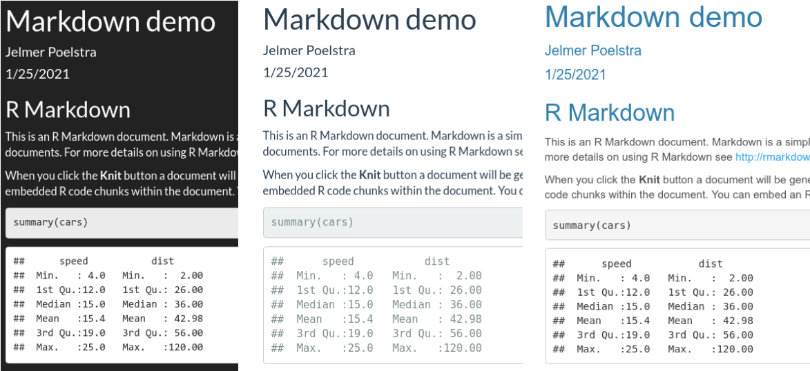
theme options: darkly, flatly, and cerulean.
IV: R Markdown and RStudio
The RMarkdown ecosystem of packages is being developed by RStudio, so it should come as no surprise that the RStudio IDE has some nice RMarkdown functionality.
Knitting and previewing your document
The process of rendering an R Markdown file into another format, as specified by the YAML header, is called knitting. We already saw the button to knit the current document (keyboard shortcut: Cmd/Ctrl+Shift+K).
If you get preview pop-up windows in RStudio, click the cog wheel icon next to the Knit button, and then select “Preview in Viewer Pane”.
Instead of knitting the entire document, you can also run individual code chunks using the green “play button” (or Cmd/Ctrl+Shift+Enter), or all code chunks up until the current one (button to the left of the play button).
For a live preview (!) of R Markdown output for your active document,
use the infinite moon reader from the xaringan package:
install.packages("xaringan")

# Simply running the function without arguments will start the preview:
xaringan::inf_mr()

# To shut down the preview server, if needed, run `servr::daemon_stop()`
Visual Markdown Editor
If your RStudio version is at least 1.4 (Click Help => About RStudio), which was released last fall, you can also use the Visual Markdown Editor.
This makes writing in R Markdown almost like using a word processor, and also includes many other features such as better citation support with Zotero integration. Read more about the visual editor here.
To switch between the visual editor and regular (“source”) editing mode, click the A-shaped ruler button in the top-right corner or press Cmd/Ctrl+Shift+F4.
This is what our document looks like in the visual editor – kind of intermediate between the raw R Markdown and the rendered output:
V: A single source doc, many output formats!
One of the greatest features of R Markdown is that you can output to many formats. So from one source document, or very similar variants, you can create completely different output depending on what you need.
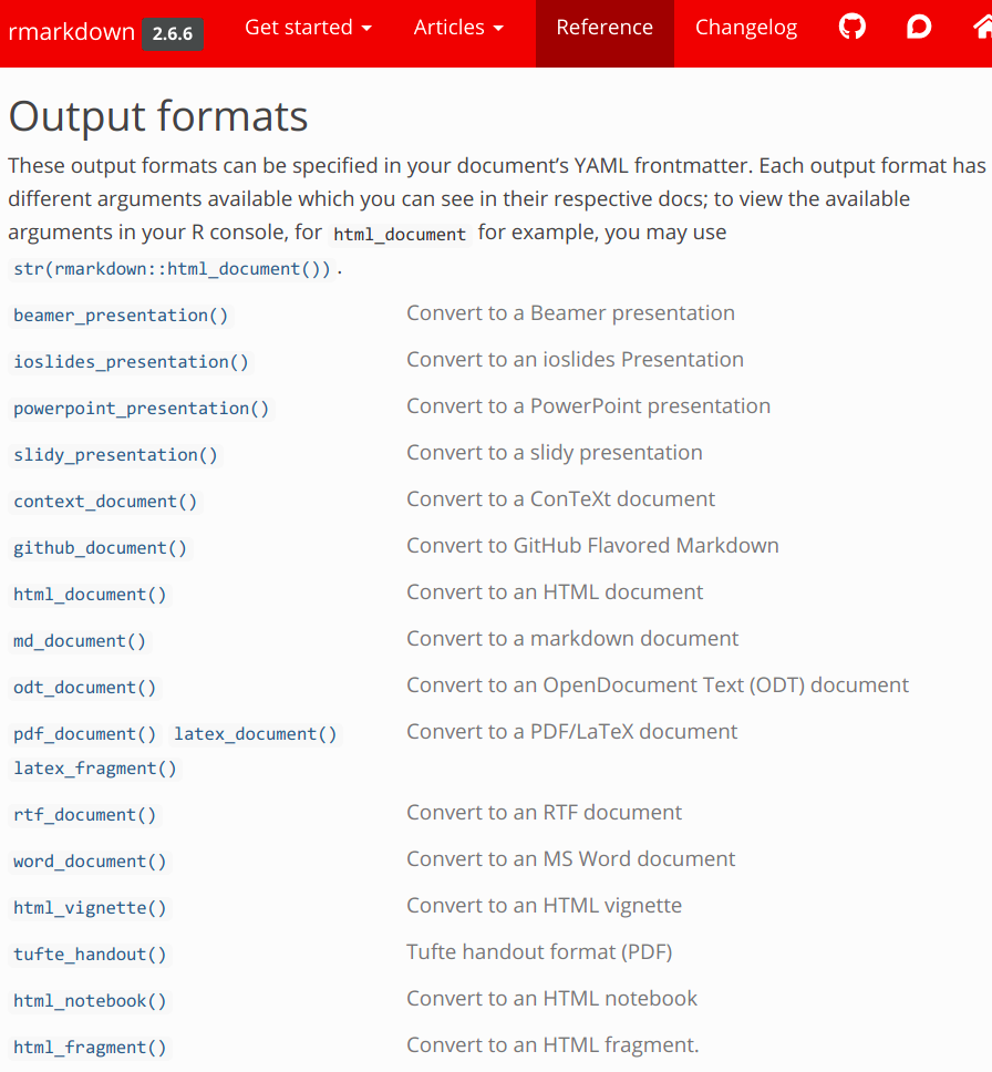
Built-in output formats
The built-in output formats, which can be used with just the rmarkdown package, are listed below. These include HTML, PDF, Word, PowerPoint, and different HTML slide show formats!
Extension output formats
It’s worth highlighting a few of the output formats that can be used with the following packages in the R Markdown ecosystem:
-
distill – An output format geared towards technical content, e.g. with extended support for equations, citations, and footnotes. Can also create websites.
-
rticles – R Markdown templates to format output for specific scientific journals.
-
flexdashboard – Create interactive “dashboards” to present data.
-
bookdown – A book format, the R Markdown book is an example.
-
xaringan – Create fancier presentation slides thanks to a JavaScript library.
Starting to use these and other output formats is often as simple as changing the YAML header:
---
output: distill::distill_article
---
Breakout rooms!
In the exercises, we will work with an .Rmd file that you can download as follows:
# dir.create("S07")     # You should have already done this

# Save the URL for the Rmd file:
todays_rmd <- 'https://raw.githubusercontent.com/biodash/biodash.github.io/master/content/codeclub/07_rmarkdown/penguins.Rmd'

# Download the Rmd file:
download.file(url = todays_rmd, destfile = 'S07/penguins.Rmd')
Next, open the document in RStudio, and fire up the infinite moon reader:
# install.packages("xaringan")

xaringan::inf_mr()
This way, you will be able to nearly instantaneously see the effect of your changes: save the document whenever you want the server to update.
You can use either the “visual editor” or the regular (“source”) editor – and you could also start by compating the two.
Exercise 1: Output formatting with YAML
In this exercise, you will fiddle with the YAML header to modify aspects of the html_document output format:
-
Add a
themekey tohtml_output, and try a few of the available value options ("default", “cerulean”, “journal”, “flatly”, “darkly”, “readable”, “spacelab”, “united”, “cosmo”, “lumen”, “paper”, “sandstone”, “simplex”, “yeti").Determine, once and for all, what the best theme is.
-
Try some of the other options mentioned above (
code_download,code_folding,toc,toc_float,toc_depth,df_print), and look at the effects on the rendered output.
Hints (click here)
-
To add options to
html_documentin the YAML header, you’ll need to go fromoutput: html_documenton a single line, to a multi-line format with indentation, and with a colon added afterhtml_document:output: html_document: <option>
Solutions (click here)
- An example YAML header with several options added:
---
title: "Penguins, demystified."
author: "Jelmer Poelstra"
date: "1/29/2021"
output:
  html_document:
    theme: flatly
    toc: true
    toc_float: true
    toc_depth: 5
    number_sections: true
    code_download: true
    code_folding: hide
    df_print: kable
---
Exercise 2: Code chunks
Our output document looks nice, but there is plenty of room for improvement. In this exercise, we’ll refine the output using code chunk options.
Before you start, take another look at the box Code chunk options above.
-
Did you notice those messages (when the tidyverse is loaded) and warnings (for the two plots) in the output? Let’s get rid of those all at once: suppress R messages and warnings for all chunks by adding arguments to the
knitr::opts_chunk$set()function in the first code chunk. -
Currently, the code line in the
install-packagecode chunk is commented out to avoid the code from running, while still printing it. Try to accomplish this using a code chunk option instead, so you can uncomment the line. -
We do want to print the code in some cases, but not in others. For the chunk labeled
print-tibble, which printspenguins, alter the settings such that the code is no longer printed. -
Our first figure is kind of squished, and the point and font sizes are perhaps too large. Compare this with the second figure, which has a different setting only for
out.width.Play around with the values for the three options that are already in the code chunks (
fig.width,out.width, andfig.asp), for one or both figures, see what the effects are, and try to make some improvements.Do you understand the difference between the two methods to indicate the figure size (
fig.widthandout.width)? -
Insert a new code chunk that prints the
penguins_rawtibble in some way (this is available in your environment).
Hints (click here)
-
To suppress messages and warnings throughout:
Addmessage=FALSEandwarnings=FALSEinsideknitr::opts_chunk$set()in thesetupchunk. -
To avoid running the code:
Useeval=FALSEin the header of theinstall-packagecode chunk. -
To avoid printing the code:
Use theechooption in the header of theprint-tibblecode chunk. -
Figure sizing:
There are two types of sizes that you can set: the size at which R creates figures (fig.widthandfig.height), and the size at which the figures are inserted in the document (out.widthandout.height). The former will effectively only control relative font and point sizes, whereas the latter controls the “actual” / final size. For more details and advice, see this section in R for Data Science.The aspect ratio (
fig.asp) is height/width, so a value smaller than one creates a wide figure and a value larger than one creates a narrow figure.Here, we’ve been setting width only – you can also set
fig.heightandout.height, but these options become redundant when you set the width and the aspect ratio.
Solutions (click here)
-
To suppress messages and warnings throughout:
knitr::opts_chunk$set(echo = TRUE, message = FALSE, warning = FALSE) -
To avoid running the code:
{r install-package, eval=FALSE} -
To avoid printing the code:
{r print-tibble, echo=FALSE} -
Figure sizing:
Example settings for better-sized figures –
{r plot-bills, out.width="80%", fig.width=6, fig.asp=0.7} -
A code chunk to print the
penguins_rawtibble (replace single quotes by backticks):
'''{r}
penguins_raw
'''
Bonus 1: Markdown and inline code
The formatting for the prose in our document could also be improved. For instance:
-
Use inline code formatting in a couple of cases where this is appropriate.
-
Instead of simply saying “8 variables (n = 344 penguins)” (under the Summary of the dataset" heading), use inline R code that makes these calculations and print the results.
-
Try a couple of other things: heading levels (one of them is currently not right!), italic text, bold text, and/or ordered (numbered) and unordered (bulleted) lists.
Hints (click here)
-
Simply put backticks around the inline text you want have formatted as code. You can do this, for instance, for mentions of
palmerpenguins::penguins. -
For inline code that runs, use
`r my-code`.The number of variables and penguins in the penguin dataset are the number of columns and rows, respectively, in the
penguintibble.
Solutions (click here)
Inline calculation of the number of variables and penguins:
[...] that contains `r ncol(penguins)` variables
(n = `r nrow(penguins)` penguins).
Bonus 2: Other output formats
Try one or more output formats other than html_document, see this website for the list of available options. If you want to try presentations, note that three dashes --- are used to separate slides.
It might be confusing that on the website linked to above (see also the screenshot in section V), the output formats are listed functions (html_document() rather than html_document) – but this is simply because under the hood, these functions are called via the YAML header.
Go further
Pitfalls / Tips
-
The working directory
By default, the working directory for an R Markdown document is the directory in which the file resides.This can be a bit annoying if you’re used to using your project’s root directory as your working directory (which you should be) and the R Markdown file is not in the project’s root directory (which it probably shouldn’t be). Nevertheless, simply using
../notation to move one or two directories up should generally work.If you really need to set a different working directory, you should be aware that surprisingly, setting the working directory with
setwd()in a code chunk is not persistent across code chunks. To set a different working directory for the entire document, useknitr::opts_knit$set(root.dir = '/my/working/dir')in a setup chunk. -
Chunk labels
Chunk labels are optional but if you do give them, note that they have to be unique: the document will fail to render if have two chunks with the same label. Also, avoid using spaces and underscores in the labels (good-chunk-label,bad chunk label,bad_chunk_label).
Tables
-
Tables produced by Markdown text
The syntax for basic Markdown tables is as follows:| Time | Session | Topic | |:--------------|:-------:|---------:| | _left_ | _center_| _right_ | | Wed 5 pm | 1 | Getting started | | Fri 3 pm | | | | Wed 5 pm | 2 | *dplyr* | | Fri 3 pm | | *Break* |Time Session Topic left center right Wed 5 pm 1 Getting started Fri 3 pm Wed 5 pm 2 dplyr Fri 3 pm Break In the Visual Markdown editor in RStudio, you can simply insert a table with a little dialogue box after clicking
Table=>Insert Table. -
Tables (dataframes) produced by R code
Usingkable(my_df)in a code chunk will create nicer output for individual dataframes (recall thedf_print: kableYAML option for document-wide “kable” printing).There are many packages available for more advanced options, such as GT, DT, and reactable.
Websites
Note that rmarkdown::render_site() can create simple websites that connects multiple pages with a navigation bar. All you need is a simple YAML file called _site.yml with some settings, and a file for the front page which needs to be called index.Rmd. See here in the R Markdown book for more details.
Options with more features, like a blog, are distill websites, and the blogdown package for Hugo sites.
Further resources
- Free online books by the primary creator of R Markdown and other authors:
- RStudio’s 5-page R Markdown Reference PDF
- RStudio’s R Markdown Cheatsheet
- RStudio R Markdown lessons
- Markdown tutorial