Code Club S02E04: Intro to the Tidyverse (Part 1)
Tidyverse, the pipe, filter, select, and 🐧
 Artwork by @allison_horst
Prep homework
Basic computer setup
-
If you didn’t already do this, please follow the Code Club Computer Setup instructions, which also has pointers for if you’re new to R or RStudio.
-
If you’re able to do so, please open RStudio a bit before Code Club starts – and in case you run into issues, please join the Zoom call early and we’ll troubleshoot.
Getting started
Now that you are familiar with the basics of RMarkdown season 1 and season 2, I put together a RMarkdown file you can download which has the content for today’s Code Club.
Download today’s content
Click here to get an Rmd (optional)
# directory for Code Club Session 2:
dir.create("S02E04")

# directory for our script
# ("recursive" to create two levels at once.)
dir.create("S02E04/Rmds/")

# save the url location for today's script
todays_Rmd <- "https://raw.githubusercontent.com/biodash/biodash.github.io/master/content/codeclub/S02E04_tidyverse-intro-part1/intro-to-tidyverse1.Rmd"

# indicate the name of the new Rmd file
intro_tidyverse1 <- "S02E04/Rmds/intro-to-tidyverse1.Rmd"

# go get that file!
download.file(url = todays_Rmd,
              destfile = intro_tidyverse1)
What will we go over today
- What is the tidyverse and why would I want to use it?
- Understanding how to use “the pipe”
%>% - Using
filter()- picks observations (i.e., rows) based on their values - Using
select()- picks variables (i.e., columns) based on their names
1 - What is the tidyverse, and how do I use it?
The tidyverse is a collection of R packages that are designed for data science. You can certainly use R without using the tidyverse, but it has many packages that I think will make your life a lot easier. The popular package ggplot2 is a part of the core tidyverse, which we have talked about in previous Code Clubs (intro, intro2, maps, and ggplotly), and will talk about in future sessions as well.
Packages contain shareable code, documentation, tests, and data. One way to download packages is using the function install.packages() which will allow you to download packages that exist within the Comprehensive R Archive Network, or CRAN. There are packages that exist outside CRAN but that is a story for another time.
Before we talk more about the tidyverse, let’s download it. We only need to do this once.
install.packages("tidyverse")To use any of the packages within the tidyverse, we need to call them up using library() anytime we want to use the code embedded within them.
library(tidyverse)
#> ── Attaching packages ─────────────────────────────────────── tidyverse 1.3.1 ──
#> ✔ ggplot2 3.3.3     ✔ purrr   0.3.4
#> ✔ tibble  3.1.4     ✔ dplyr   1.0.7
#> ✔ tidyr   1.1.3     ✔ stringr 1.4.0
#> ✔ readr   1.4.0     ✔ forcats 0.5.1
#> ── Conflicts ────────────────────────────────────────── tidyverse_conflicts() ──
#> ✖ dplyr::filter() masks stats::filter()
#> ✖ dplyr::lag()    masks stats::lag()
Let’s look at this message, we can see that there are eight “attaching packages” as part of the “core” set of tidyverse.
We see that there are some conflicts, for example, there is a function called filter() (which we will talk about today) that is part of dplyr (a tidyverse package) that is masking another function called filter() within the stats package (which loads with base R).
The conflict arises from the fact that there are now two functions named filter(). After loading the tidyverse, the default filter() will be that from dplyr. If we want explcitly to use the filter() function from stats, we can do that using the double colon operator :: like this: stats::filter().
Now this is fine for us right now, so there is nothing to do, but it is a good habit to get into reading (and not ignoring) any warnings or messages that R gives you. (It is trying to help!)
Remember, you can learn more about any package by accessing the help documentation. The help will pop up in the Help tab of the bottom right quadrant of RStudio when you execute the code below.
?tidyverse
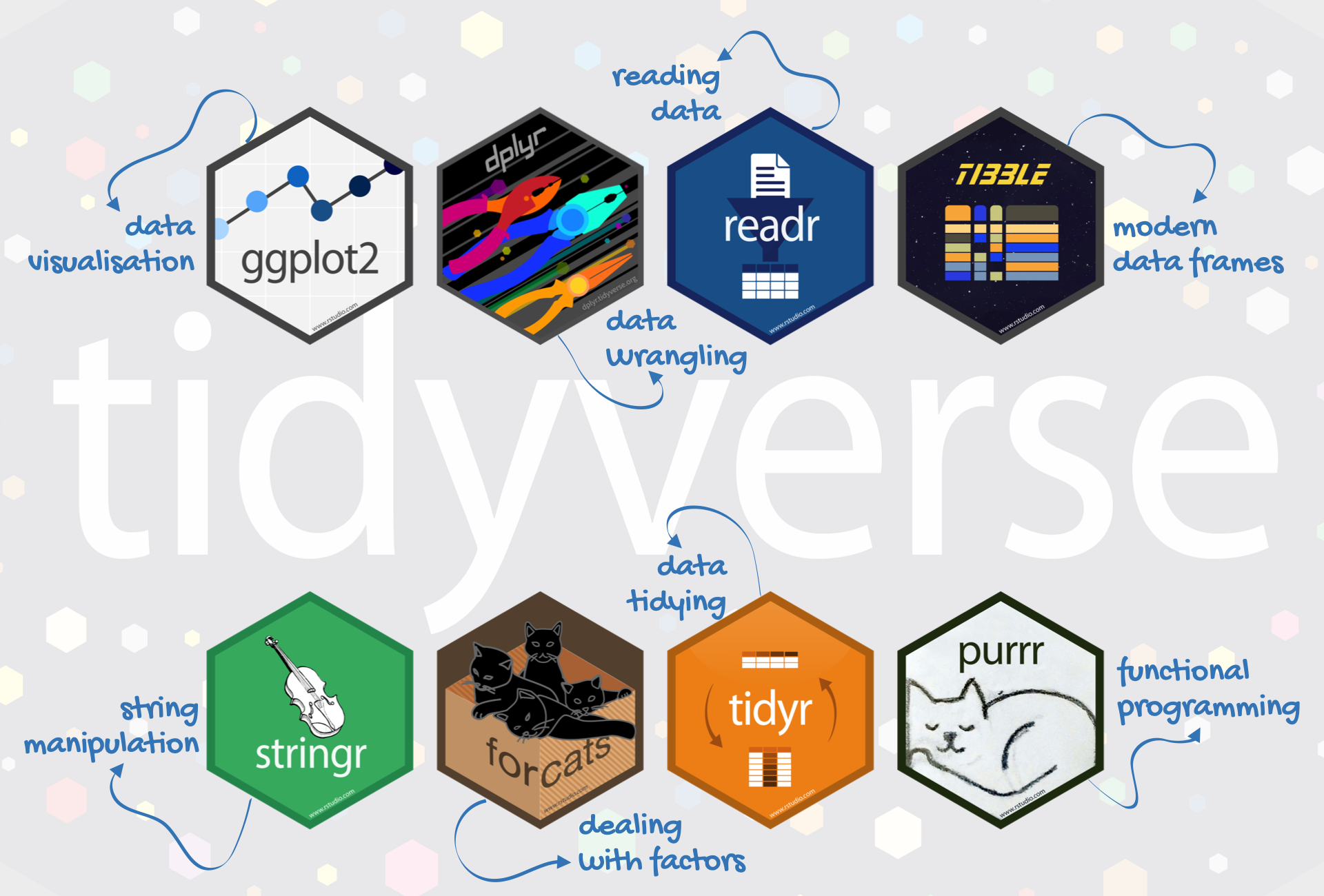
Below is a quick description of what each package is used for.
dplyr: for data manipulationggplot2: a “grammar of graphics” for creating beautiful plotsreadr: for reading in rectangular data (i.e., Excel-style formatting)tibble: using tibbles as modern/better dataframesstringr: handling strings (i.e., text or stuff in quotes)forcats: for handling categorical variables (i.e., factors) (meow!)tidyr: to make “tidy data”purrr: for enhancing functional programming (also meow!)
If you’re not understanding what some of this means, that’s totally fine.
There are more tidyverse packages outside of these core eight, and you can see what they are below.
tidyverse_packages()
#>  [1] "broom"         "cli"           "crayon"        "dbplyr"
#>  [5] "dplyr"         "dtplyr"        "forcats"       "googledrive"
#>  [9] "googlesheets4" "ggplot2"       "haven"         "hms"
#> [13] "httr"          "jsonlite"      "lubridate"     "magrittr"
#> [17] "modelr"        "pillar"        "purrr"         "readr"
#> [21] "readxl"        "reprex"        "rlang"         "rstudioapi"
#> [25] "rvest"         "stringr"       "tibble"        "tidyr"
#> [29] "xml2"          "tidyverse"
tl;dr Tidyverse has a lot of packages that make data analysis easier. None of them are ‘required’ to do data analysis, but many tidyverse approaches you’ll find easier than using base R.
You can find here some examples of comparing tidyverse and base R syntax.
2 - Using the pipe %>%
The pipe operator %>% is a tool that is used for expressing a series of operations. It comes from the magrittr package, and is loaded automatically when you load the tidyverse.
The purpose of the pipe is to allow you to take the output of one operation and have it be the starting material of the next step. It also (hopefully) makes your code easier to read and interpret.
Let’s get set up and grab some data so that we have some material to work with.

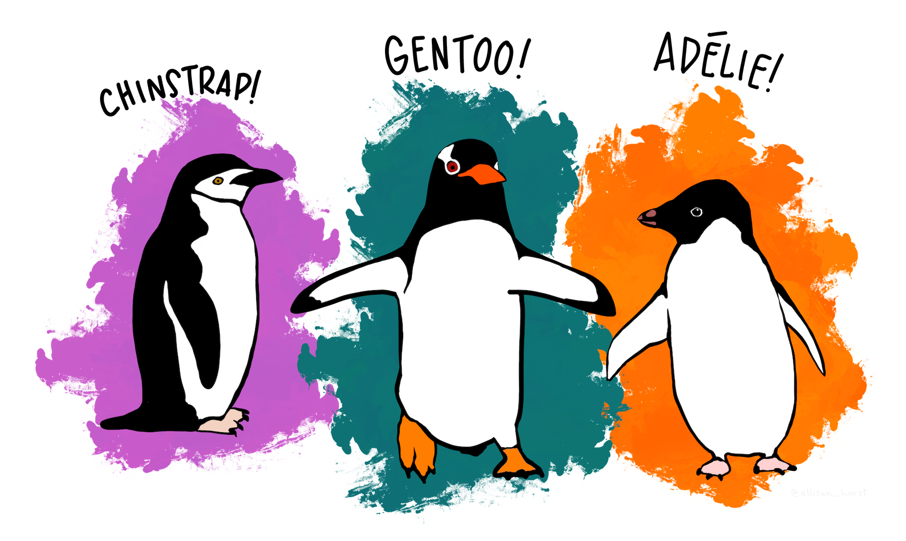
Illustration by Allison Horst
We are going to use a package called palmerpenguins which has some fun 🐧 data for us to play with. To get this data, we need to install the palmerpenguins package.
install.packages(palmerpenguins)palmerpenguins is a package developed by Allison Horst, Alison Hill and Kristen Gorman, including a dataset collected by Dr. Kristen Gorman at the Palmer Station Antarctica, as part of the Long Term Ecological Research Network. It is a nice, relatively simple dataset to practice data exploration and visualization in R. Plus the penguins are v cute.
Then, to use the package, we need to use the function library() to call the package up in R.
The data we will use today is called penguins.
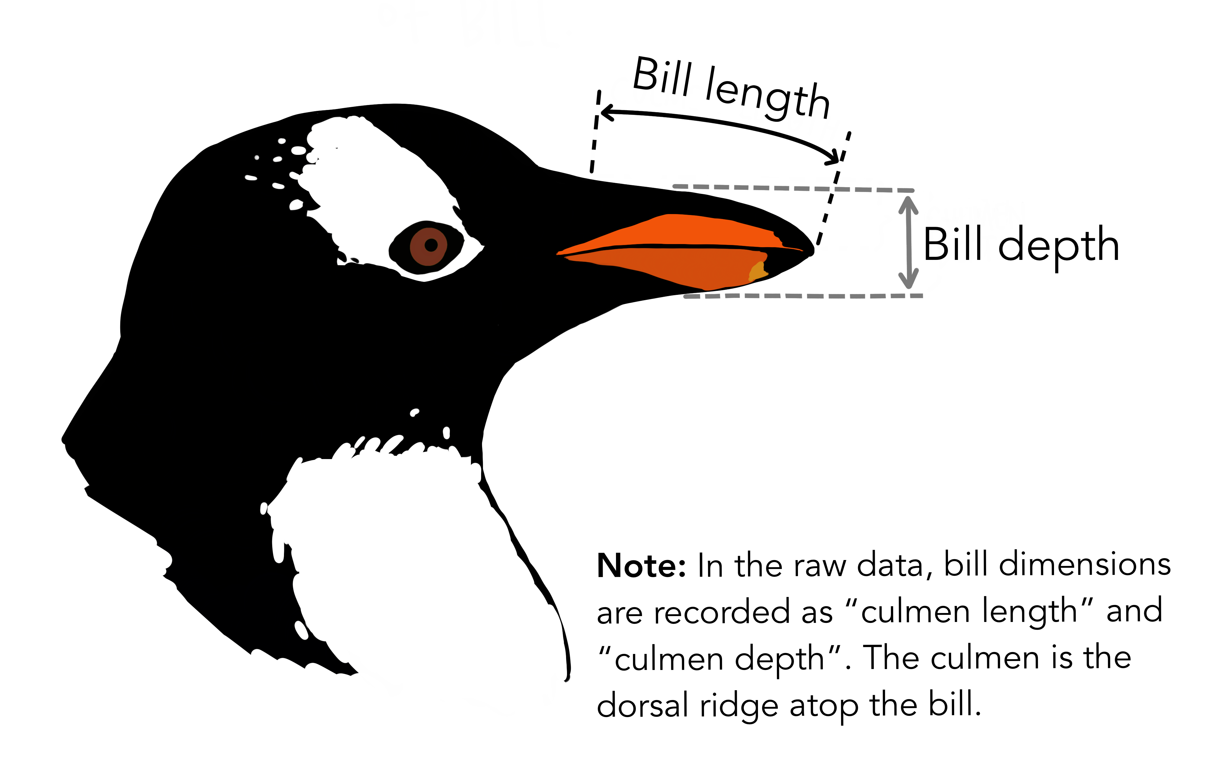
Illustration by Allison Horst
# look at the first 6 rows, all columns
head(penguins)
#> # A tibble: 6 × 8
#>   species island bill_length_mm bill_depth_mm flipper_length_… body_mass_g sex
#>   <fct>   <fct>           <dbl>         <dbl>            <int>       <int> <fct>
#> 1 Adelie  Torge…           39.1          18.7              181        3750 male
#> 2 Adelie  Torge…           39.5          17.4              186        3800 fema…
#> 3 Adelie  Torge…           40.3          18                195        3250 fema…
#> 4 Adelie  Torge…           NA            NA                 NA          NA NA
#> 5 Adelie  Torge…           36.7          19.3              193        3450 fema…
#> 6 Adelie  Torge…           39.3          20.6              190        3650 male
#> # … with 1 more variable: year <int>

# check the structure of penguins_data
# glimpse() which is a part of dplyr functions
# similarly to str() and can be used interchangeably
glimpse(penguins)
#> Rows: 344
#> Columns: 8
#> $ species           <fct> Adelie, Adelie, Adelie, Adelie, Adelie, Adelie, Adel…
#> $ island            <fct> Torgersen, Torgersen, Torgersen, Torgersen, Torgerse…
#> $ bill_length_mm    <dbl> 39.1, 39.5, 40.3, NA, 36.7, 39.3, 38.9, 39.2, 34.1, …
#> $ bill_depth_mm     <dbl> 18.7, 17.4, 18.0, NA, 19.3, 20.6, 17.8, 19.6, 18.1, …
#> $ flipper_length_mm <int> 181, 186, 195, NA, 193, 190, 181, 195, 193, 190, 186…
#> $ body_mass_g       <int> 3750, 3800, 3250, NA, 3450, 3650, 3625, 4675, 3475, …
#> $ sex               <fct> male, female, female, NA, female, male, female, male…
#> $ year              <int> 2007, 2007, 2007, 2007, 2007, 2007, 2007, 2007, 2007…
Okay now we have a sense of what the penguins dataset is.
If we want to know how many penguins there are of each species we can use the function count(). In the count() function, the first argument is the dataset, and the next argument is what you want to be counted. You can always learn more about the arguments and syntax of functions by using ?yourfunction() or googling for the documentation. This is the non-pipe approach.
count(penguins, species)
#> # A tibble: 3 × 2
#>   species       n
#>   <fct>     <int>
#> 1 Adelie      152
#> 2 Chinstrap    68
#> 3 Gentoo      124
Alternatively, we can use the pipe to send penguins forward through a series of steps. For example, we can use the function count() to figure out how many of each penguin species there are in our dataset.
penguins %>% # take penguins_data
  count(species) # count how many of each species there is
#> # A tibble: 3 × 2
#>   species       n
#>   <fct>     <int>
#> 1 Adelie      152
#> 2 Chinstrap    68
#> 3 Gentoo      124
Comparing to base R
A main benefit of the pipe is readability, and also the ability to “pipe” many things together (which we are not doing with count()).
I want to stress that everything you can do with the tidyverse you can also do using base R. I tend to think the tidyverse is more intuitive than base R, which is why we have elected to teach it here first. Here you can find a bunch of examples comparing tidyverse to base R equivalent syntax. Here is an interesting blogpost on the topic if this is really keeping you up at night.
I am going to show you an example of a place I think the pipe really shines, don’t worry if you don’t understand all the syntax, I just want you to see how the pipe can be used.
penguins %>%
  drop_na() %>% # drop missing values listed as NA
  group_by(species) %>% # group by species
  summarize(mean_mass = mean(body_mass_g)) # summarize mass into new column called
#> # A tibble: 3 × 2
#>   species   mean_mass
#>   <fct>         <dbl>
#> 1 Adelie        3706.
#> 2 Chinstrap     3733.
#> 3 Gentoo        5092.
We are going to continue to use the pipe %>% as we practice with some new dplyr functions.
Breakout session 1 - install tidyverse, use the pipe
In your breakout sessions, make sure that you each have the tidyverse installed and loaded.
Solution (click here)
install.packages("tidyverse")
install.packages("dplyr") # this is the only one of the 8 tidyverse packages we will use today

library(tidyverse)
Occasionally we see people who are having tidyverse install issues, if this happens to you, please read the warning that R gives you, you may need to download an additional package to get it to work. If you have trouble, first try restarting your R session and see if that helps, or reach out to one of the organizers or one of your fellow codeclubbers.
We will practice using the pipe. In S02E02, Mike introduced you to some new functions in Exercise 6. Take the dataset penguins and use the pipe to determine the dimensions of the dataframe.
Solution (click here)
penguins %>%
  dim()
#> [1] 344   8
This means the dataframe is 344 rows and 8 columns in size.
Take the dataset penguins and use the pipe to determine the names of the columns of the dataframe.
Solution (click here)
penguins %>%
  names()
#> [1] "species"           "island"            "bill_length_mm"
#> [4] "bill_depth_mm"     "flipper_length_mm" "body_mass_g"
#> [7] "sex"               "year"

# the same
penguins %>%
  colnames()
#> [1] "species"           "island"            "bill_length_mm"
#> [4] "bill_depth_mm"     "flipper_length_mm" "body_mass_g"
#> [7] "sex"               "year"
These are the names of our 8 columns.
3 - Using select()
It has been estimated that the process of getting your data into the appropriate formats takes about 80% of the total time of analysis. I find that getting data into a format that enables analysis often trips people up more than doing the actual analysis. The tidyverse package dplyr has a number of functions that help in data wrangling.
The first one we will talk about is select(). Tidyverse is nice in that the functions are very descriptive and intuitive as to what they do: select() allows you to pick certain columns to be included in your data frame.
Let’s try out both the %>% and select(). Let’s make a new dataframe from penguins that contains only the variables species, island and sex.
penguins_only_factors <- penguins %>%
  select(species, island, sex)
Did it work?
head(penguins_only_factors)
#> # A tibble: 6 × 3
#>   species island    sex
#>   <fct>   <fct>     <fct>
#> 1 Adelie  Torgersen male
#> 2 Adelie  Torgersen female
#> 3 Adelie  Torgersen female
#> 4 Adelie  Torgersen NA
#> 5 Adelie  Torgersen female
#> 6 Adelie  Torgersen male
Let’s check the dimensions of each dataframe to make sure we have what we would expect
# what are the dimensions of penguins?
dim(penguins)
#> [1] 344   8

# what are the dimensions of penguins_only_factors?
dim(penguins_only_factors)
#> [1] 344   3
The output is ordered rows (first number) by columns (second number). Our output makes sense - we haven’t removed any observation (i.e., rows), we have only selected some of the columns that we want to work with.
What if we want to pick just the first three columns? We can do that too.
str(penguins) # what are those first three columns?
#> tibble [344 × 8] (S3: tbl_df/tbl/data.frame)
#>  $ species          : Factor w/ 3 levels "Adelie","Chinstrap",..: 1 1 1 1 1 1 1 1 1 1 ...
#>  $ island           : Factor w/ 3 levels "Biscoe","Dream",..: 3 3 3 3 3 3 3 3 3 3 ...
#>  $ bill_length_mm   : num [1:344] 39.1 39.5 40.3 NA 36.7 39.3 38.9 39.2 34.1 42 ...
#>  $ bill_depth_mm    : num [1:344] 18.7 17.4 18 NA 19.3 20.6 17.8 19.6 18.1 20.2 ...
#>  $ flipper_length_mm: int [1:344] 181 186 195 NA 193 190 181 195 193 190 ...
#>  $ body_mass_g      : int [1:344] 3750 3800 3250 NA 3450 3650 3625 4675 3475 4250 ...
#>  $ sex              : Factor w/ 2 levels "female","male": 2 1 1 NA 1 2 1 2 NA NA ...
#>  $ year             : int [1:344] 2007 2007 2007 2007 2007 2007 2007 2007 2007 2007 ...

penguins %>%
  select(species:bill_length_mm) %>% # pick columns species through bill_length_mm
  head() # you can add head() as part of your pipe!
#> # A tibble: 6 × 3
#>   species island    bill_length_mm
#>   <fct>   <fct>              <dbl>
#> 1 Adelie  Torgersen           39.1
#> 2 Adelie  Torgersen           39.5
#> 3 Adelie  Torgersen           40.3
#> 4 Adelie  Torgersen           NA
#> 5 Adelie  Torgersen           36.7
#> 6 Adelie  Torgersen           39.3
Note, in the above chunk, this new dataframe is not being saved because we have not assigned it to anything.
You could use slightly different syntax to get the same thing using an indexing approach.
penguins %>%
  select(1:3) %>% # pick columns 1-3
  head()
#> # A tibble: 6 × 3
#>   species island    bill_length_mm
#>   <fct>   <fct>              <dbl>
#> 1 Adelie  Torgersen           39.1
#> 2 Adelie  Torgersen           39.5
#> 3 Adelie  Torgersen           40.3
#> 4 Adelie  Torgersen           NA
#> 5 Adelie  Torgersen           36.7
#> 6 Adelie  Torgersen           39.3
There is also convenient shorthand for indicating what you don’t want (instead of what you do).
penguins %>%
  select(-year) %>% # all the columns except year
  head()
#> # A tibble: 6 × 7
#>   species island bill_length_mm bill_depth_mm flipper_length_… body_mass_g sex
#>   <fct>   <fct>           <dbl>         <dbl>            <int>       <int> <fct>
#> 1 Adelie  Torge…           39.1          18.7              181        3750 male
#> 2 Adelie  Torge…           39.5          17.4              186        3800 fema…
#> 3 Adelie  Torge…           40.3          18                195        3250 fema…
#> 4 Adelie  Torge…           NA            NA                 NA          NA NA
#> 5 Adelie  Torge…           36.7          19.3              193        3450 fema…
#> 6 Adelie  Torge…           39.3          20.6              190        3650 male
Embedded within select() is the column order - you can change the order by denoting the order of your columns.
penguins %>%
  select(bill_length_mm, island, flipper_length_mm) %>%
  head()
#> # A tibble: 6 × 3
#>   bill_length_mm island    flipper_length_mm
#>            <dbl> <fct>                 <int>
#> 1           39.1 Torgersen               181
#> 2           39.5 Torgersen               186
#> 3           40.3 Torgersen               195
#> 4           NA   Torgersen                NA
#> 5           36.7 Torgersen               193
#> 6           39.3 Torgersen               190
4 - Using filter()
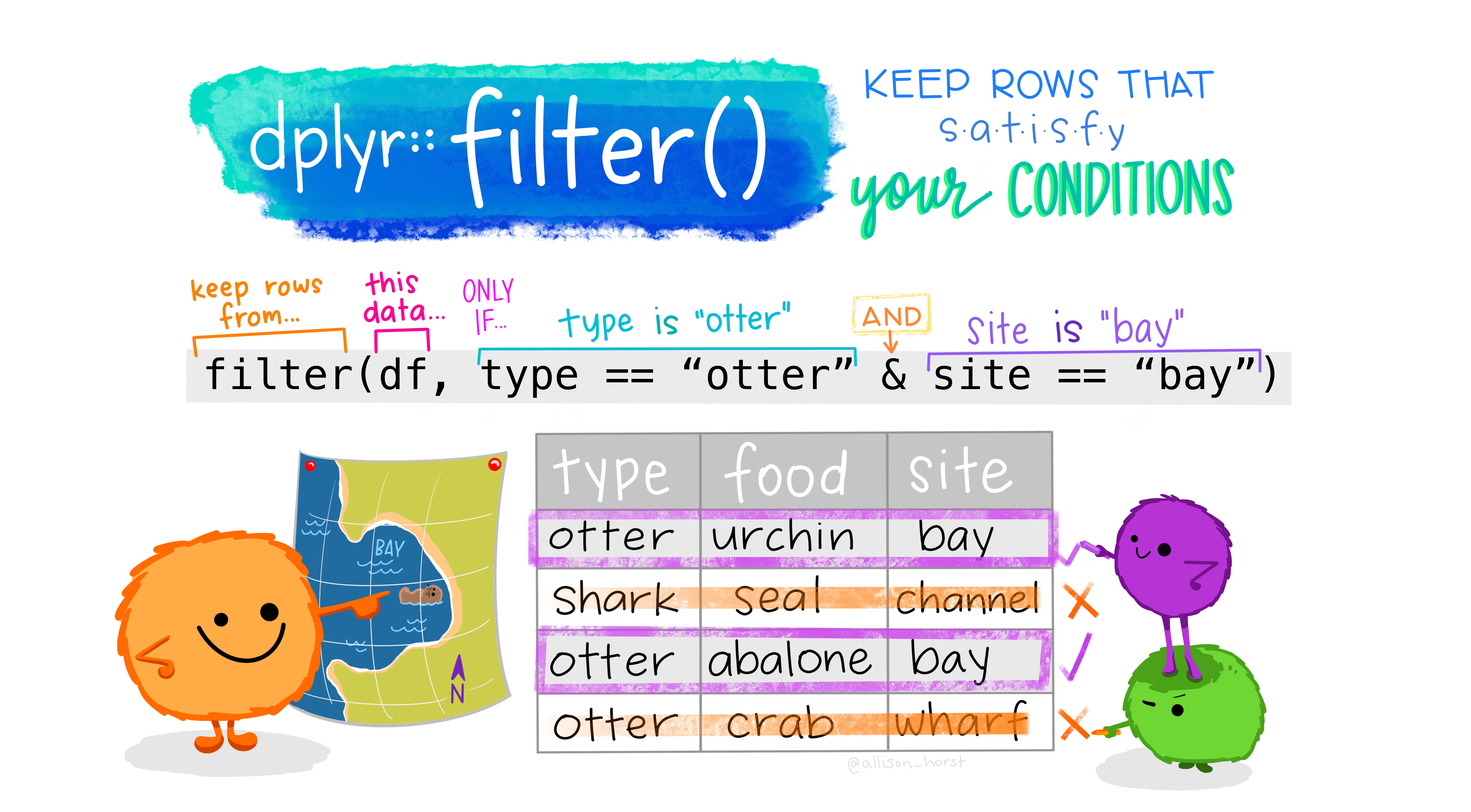
filter() allows you to pick certain observations (i.e, rows) based on their values to be included in your data frame. Let’s see it in action.
penguins_chinstrap <- penguins %>%
  filter(species == "Chinstrap") # note the double equals

# let's check that it worked
penguins_chinstrap %>%
  count(species)
#> # A tibble: 1 × 2
#>   species       n
#>   <fct>     <int>
#> 1 Chinstrap    68
We can also check to see if we got what we would expect by looking at the dimensions of both penguins and penguins_chinstrap.
Great, you can see we have kept all of the columns (denoted by the second number 8), but trimmed down the rows/observations to only the Chinstrap penguins.
You can use filter() in other useful ways too. Let’s make a new dataframe that has only the penguins that are over 5000 g.
big_penguins <- penguins %>%
  filter(body_mass_g > 5000)

# did it work?
big_penguins %>%
  select(body_mass_g) %>%
  range()
#> [1] 5050 6300

# another faster non-tidyverse way to do this
range(big_penguins$body_mass_g)
#> [1] 5050 6300
You can start stacking qualifiers to get the exact penguins you want. Let’s say we are only interested in penguins that are female and on the island Dream.
penguins %>%
  filter(sex == "female" & island == "Dream")
#> # A tibble: 61 × 8
#>    species island bill_length_mm bill_depth_mm flipper_length_mm body_mass_g
#>    <fct>   <fct>           <dbl>         <dbl>             <int>       <int>
#>  1 Adelie  Dream            39.5          16.7               178        3250
#>  2 Adelie  Dream            39.5          17.8               188        3300
#>  3 Adelie  Dream            36.4          17                 195        3325
#>  4 Adelie  Dream            42.2          18.5               180        3550
#>  5 Adelie  Dream            37.6          19.3               181        3300
#>  6 Adelie  Dream            36.5          18                 182        3150
#>  7 Adelie  Dream            36            18.5               186        3100
#>  8 Adelie  Dream            37            16.9               185        3000
#>  9 Adelie  Dream            36            17.9               190        3450
#> 10 Adelie  Dream            37.3          17.8               191        3350
#> # … with 51 more rows, and 2 more variables: sex <fct>, year <int>
There are lots of useful generic R operators that you can use inside functions like filter() including:
==: exactly equals to>=: greater than or equals to, you can also use ≥<=: less than or equals to, you can also use ≤&: and|: or!=: not equal to!x: not xis.na(): is NA (i.e. missing data)
There is a longer list of helpful select() features here.
tl;dr, select() picks columns/variables and filter() picks rows/observations.
Breakout session 2 - pipe, filter, select
Exercise 1
Make a new dataframe called penguins_new that includes only the columns with numeric or integer data.
Hints (click here)
Use str() or glimpse() to figure out which columns are numeric or integers. Then use select() to pick only the columns you want.
Solution (click here)
glimpse(penguins)
#> Rows: 344
#> Columns: 8
#> $ species           <fct> Adelie, Adelie, Adelie, Adelie, Adelie, Adelie, Adel…
#> $ island            <fct> Torgersen, Torgersen, Torgersen, Torgersen, Torgerse…
#> $ bill_length_mm    <dbl> 39.1, 39.5, 40.3, NA, 36.7, 39.3, 38.9, 39.2, 34.1, …
#> $ bill_depth_mm     <dbl> 18.7, 17.4, 18.0, NA, 19.3, 20.6, 17.8, 19.6, 18.1, …
#> $ flipper_length_mm <int> 181, 186, 195, NA, 193, 190, 181, 195, 193, 190, 186…
#> $ body_mass_g       <int> 3750, 3800, 3250, NA, 3450, 3650, 3625, 4675, 3475, …
#> $ sex               <fct> male, female, female, NA, female, male, female, male…
#> $ year              <int> 2007, 2007, 2007, 2007, 2007, 2007, 2007, 2007, 2007…

penguins_new <- penguins %>%
  select(bill_length_mm:body_mass_g, year)

# check to see if it worked
head(penguins_new)
#> # A tibble: 6 × 5
#>   bill_length_mm bill_depth_mm flipper_length_mm body_mass_g  year
#>            <dbl>         <dbl>             <int>       <int> <int>
#> 1           39.1          18.7               181        3750  2007
#> 2           39.5          17.4               186        3800  2007
#> 3           40.3          18                 195        3250  2007
#> 4           NA            NA                  NA          NA  2007
#> 5           36.7          19.3               193        3450  2007
#> 6           39.3          20.6               190        3650  2007
Getting fancy with some more advanced options
# this works too
penguins_new2 <- penguins %>%
  select(ends_with("mm"), body_mass_g, year)

# this works three
penguins_new3 <- penguins %>%
  select(where(is.numeric) | where(is.integer))

# are they all the same?
all.equal(penguins_new2, penguins_new3)
#> [1] TRUE
Exercise 2
Make a new dataframe called penguins_adelie_female that includes only the female penguins that are of the species Adelie.
Hints (click here)
Use filter() to set which penguins you want to keep. Use the %>% and count() to make sure what you did worked.
Solution (click here)
penguins_adelie <- penguins %>%
  filter(species == "Adelie" & sex == "female")

# check to see if it worked
penguins_adelie %>%
  count(species, sex)
#> # A tibble: 1 × 3
#>   species sex        n
#>   <fct>   <fct>  <int>
#> 1 Adelie  female    73
Exercise 3
Make a new dataframe called penguins_dream_or_2007 that includes only the penguins on the island dream, or from the year 2007. Then make sure the dataframe only contains those variables you have filtered on.
Hints (click here)
Use filter() to set which penguins you want to keep. Use the %>% and select() to construct your new dataframe.
Solution (click here)
penguins_dream_or_2007 <- penguins %>%
  filter(island == "Dream" | year == "2007") %>%
  select(island, year)

head(penguins_dream_or_2007)
#> # A tibble: 6 × 2
#>   island     year
#>   <fct>     <int>
#> 1 Torgersen  2007
#> 2 Torgersen  2007
#> 3 Torgersen  2007
#> 4 Torgersen  2007
#> 5 Torgersen  2007
#> 6 Torgersen  2007

# did it work?
penguins_dream_or_2007 %>%
  count(island, year)
#> # A tibble: 5 × 3
#>   island     year     n
#>   <fct>     <int> <int>
#> 1 Biscoe     2007    44
#> 2 Dream      2007    46
#> 3 Dream      2008    34
#> 4 Dream      2009    44
#> 5 Torgersen  2007    20
Further reading
There are many good (free) references for the tidyverse, including the book R for Data Science by Hadley Wickham and Garrett Grolemund.
The package dplyr, as part of the tidyverse has a number of very helpful functions that will help you get your data into a format suitable for your analysis.
RStudio makes very useful cheatsheets, including ones on tidyverse packages like dplyr, ggplot2, and others.