Code Club S02E03: R Markdown
Text + Code + Output
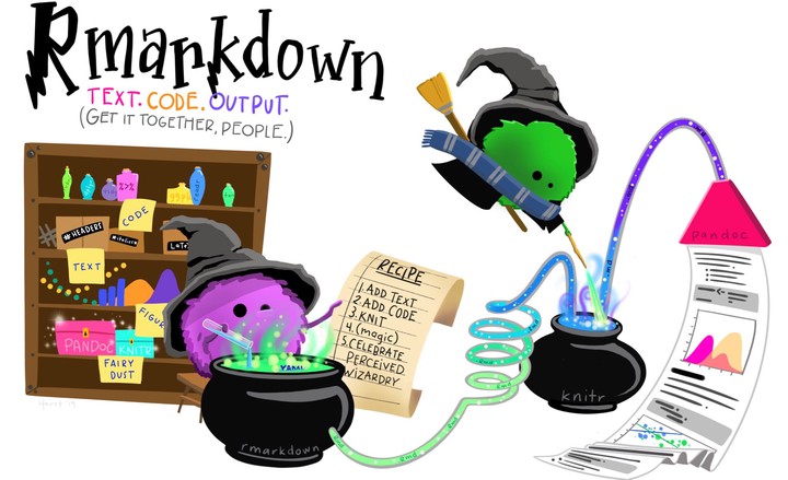 Artwork by @allison_horst
Introduction
R Markdown consists of an amazing ecosystem of R packages to produce many types of technical content. Its signature capability is that is can print formatted text, run R code, and display the results, all inside a single document. Furthermore, you can easily export this document in a large variety of formats, including HTML, PDF, Word, RTF, etc. The webpage you are looking at now was written (almost) completely in R Markdown.
At the most basic level, instead of using comments interleaved with your code in an R script:
# This is a comment
you can insert formatted text around your code in an R Markdown file. You can structure your document with headings and subheadings. You can add tables of contents. You can even generate formatted bibliographies. And the R code you insert in the document runs inside the document and the results go to the document itself, not to the console or (in the case of plots) to the Plots pane in RStudio.
This makes RMarkdown a great computer lab notebook, since you can explain what you’re doing and why (to colleagues or your future self). It’s also an example of reproducible research since you share not just a Word file, say, with example code, but an active document in which the code actually runs and the results are reproduced.
To understand R Markdown, we need to learn about three new things:
-
Markdown, a very lightweight text formatting language.
-
Code chunks, which allow us to incorporate R code that can be executed and whose results we can display in text, figures, and tables.
-
The YAML header, which encodes metadata about the output, such as the desired output format and specific formatting features.
We’ll focus on HTML output, but will also glance at other possibilities for the output format: with R Markdown, it is possible to create not just technical reports, but also slide decks, websites, books, scientific articles, dissertations, and so on.
Setup
At the core of the R Markdown ecosystem is the rmarkdown package. We need to install this but don’t need to load it:
install.packages("rmarkdown")Inside your directory for Code Club, create a folder for this week:
dir.create('S02E03')Select this folder in the Files pane. Then make this your working directory, using “Set as Working Directory” from the More options:
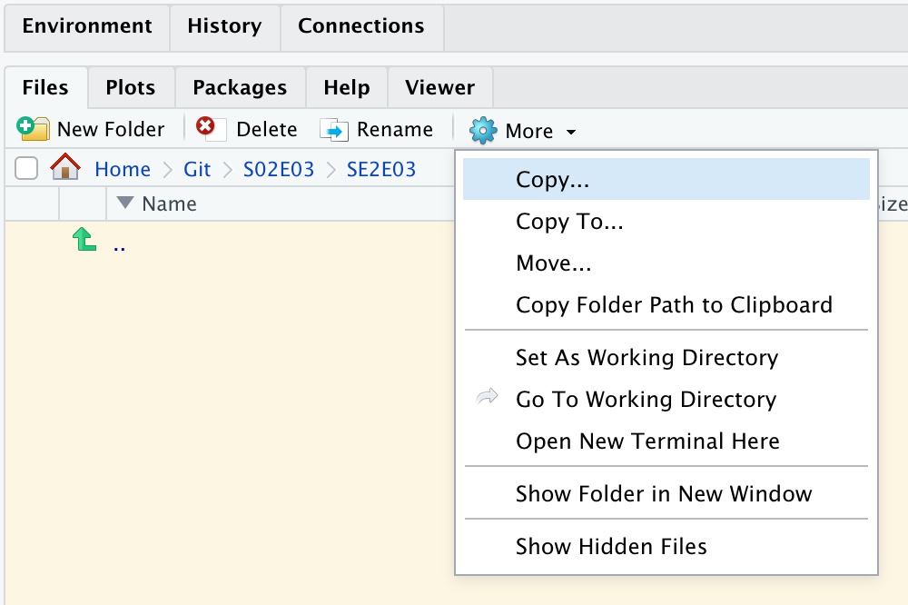
(You don’t need to do this now: we’ll make it part of the first Breakout Room in just a moment…)
First, an example
Before we go into details, let’s first see a quick demonstration of what we’re talking about. RStudio lets you create an example R Markdown document with a couple of clicks. Here are the instructions: I’ll run through them, and then we’ll open Breakout rooms so you can try it out yourself.
-
Go to
File=>New File=>R Markdown, change the Title to “Markdown demo”, and clickOK. -
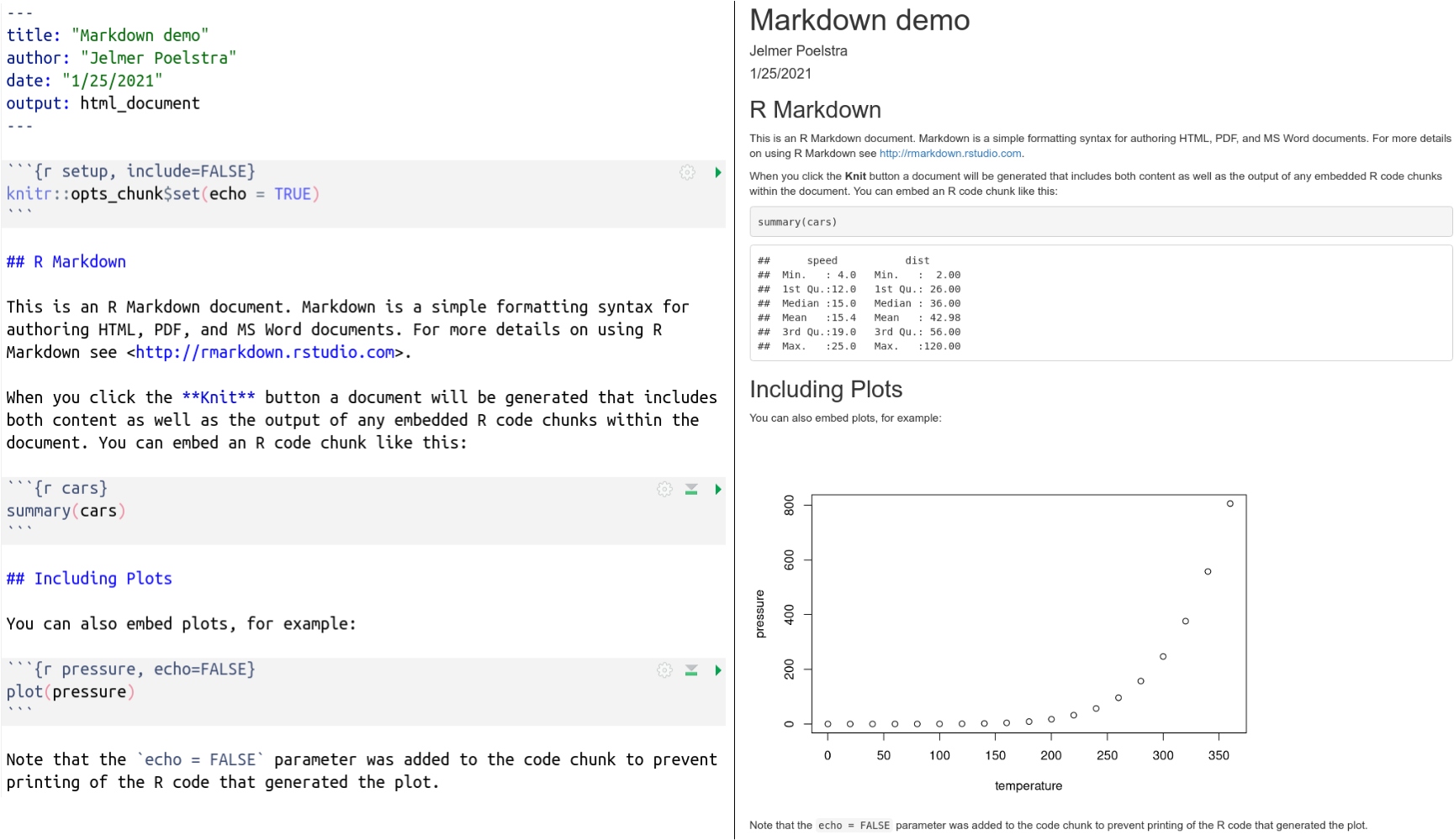
Take a look at the R Markdown document, and notice that there seems to be some sort of header bounded by three dashes (=> YAML), followed by R code wrapped in strange constructs with backticks and curly brackets (=> Code chunks), and formatted written text (=> Markdown).
-
Before we can render the output, we need to save the document. Click the
Savebutton and save the files asdemo.Rmdinside your newly created directory. -
Now click the Knit button in one of the top bars, and a document should show up in a pop-up in the Viewer pane. This is the rendered output from the R Markdown document, which is translated from Markdown into HTML behind the scenes, and displayed using a built in web-browser.
Notice that the YAML header is not printed (at least not verbatim) while some of the code is printed (some is hidden), and we also see code output, including a plot!
This is what the raw and rendered output look side-by-side:
Breakout Room 1
Work through the example above yourselves. Generate a sample R Markdown file, in the correct directory, look at the contents, and make sure you can render it on your system using the “Knit” to HTML button in the top command bar.
We’ll now talk about Markdown, code chunks, and the YAML header in turn.
I: Markdown
To fully appreciate the magic of Markdown and where it came from, it’s useful to just briefly visit the notion of a Markup language.
The original markup was done by a subeditor using a blue pencil on a handwritten or typed manuscript. This markup included typographic instructions for printing, like making a heading larger or text boldface, etc.
Computer Markup languages have the same kind of annotations, which are included in the plain text, but are visually different from the content. This marked-up text is then sent to an interpreter (e.g. a web browser, a PDF viewer, an app like Word) which renders the final document.
A large number of markup languages have been developed over the years. At current count there are about 60. This is how you would markup italic text in a small selection of them:
HTML
<i>This text is italic</i>
Word .docx
<w:t>This is italic text.</w:t>
TeX
\textit{This text is italic}
ODF text document .odt
<text:p text:style-name="P1">This text is italic.</text:p>
Rich text format .rtf
{\rtlch\ai \ltrch\loch\i\loch This text is italic.}
Some of these are more readable than others. Some are never meant to be read by humans at all! But underneath the hood every format is actually Markup.
The aim of Markdown is to create lightweight Markup language, which is easy to read and easy to write in a text editor. It embodies the principle: “make common things easy, and rare things possible”. Then we let the computer do the work of translating Markdown into various markup languages and rendering them, so we don’t have to worry about the details:
Markdown
*This text is italic.*
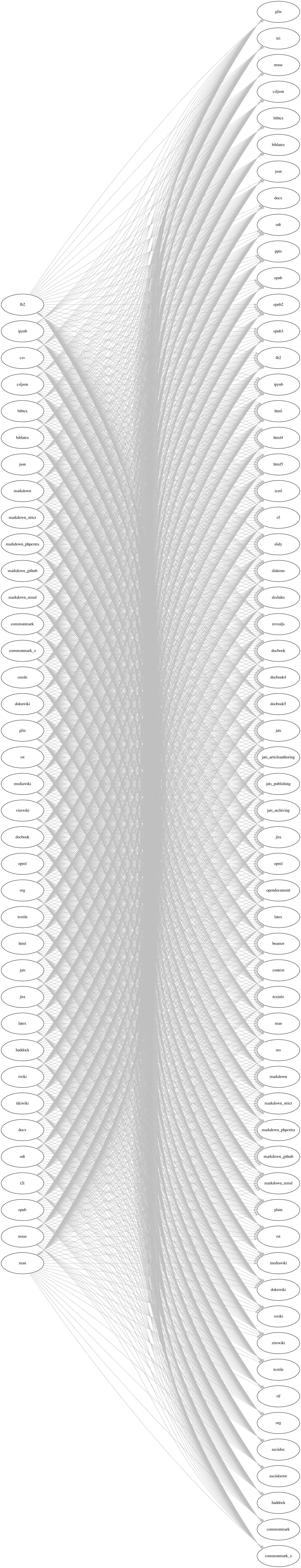
The “Swiss Army Knife” for letting the computer convert between Markup languages is Pandoc. The Pandoc site contains a graphic which shows what can be translated to what (included here just to give you a sense of the extent of this Markup world):
Click here to see the Pandoc figure
R Markdown uses Pandoc as its engine for translating Markdown to various Markup languages.
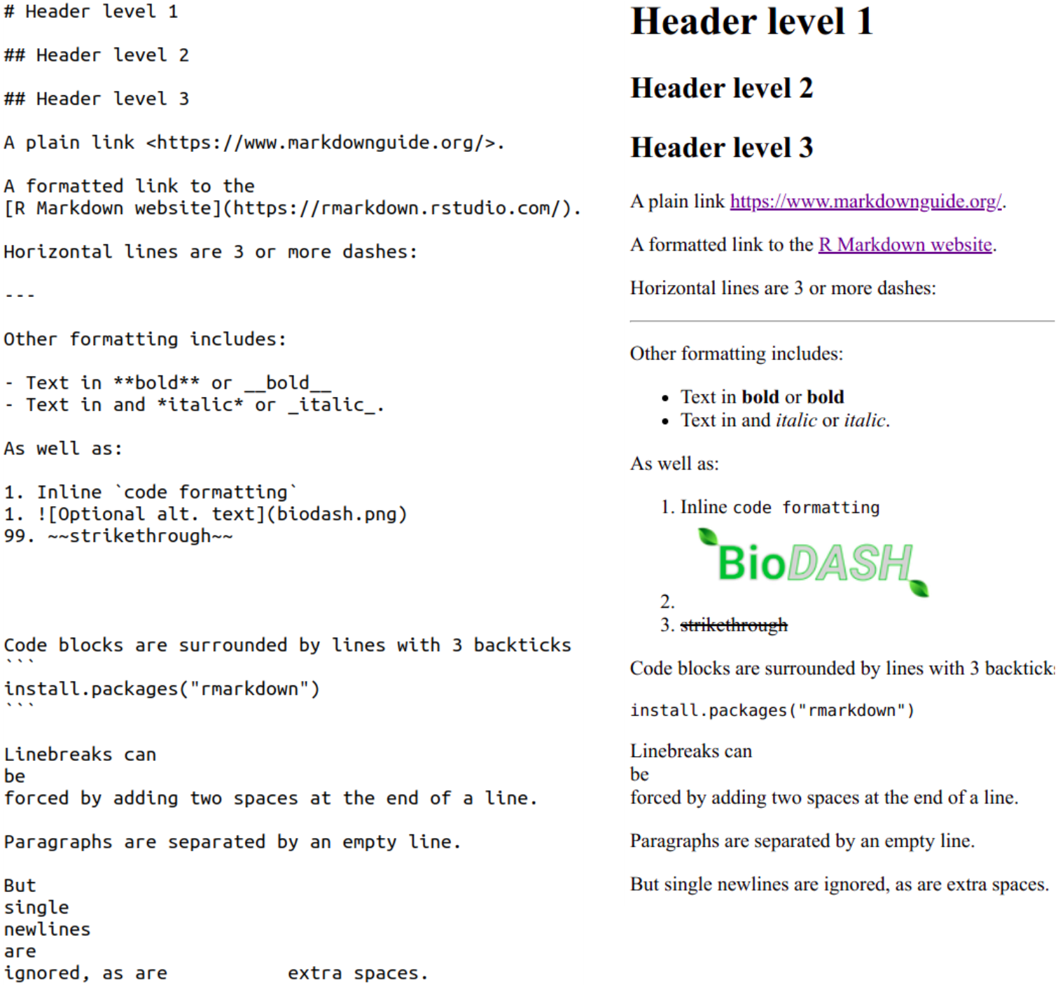
An overview of commonly used Markdown syntax
| Syntax | Result |
|---|---|
| # My Title | Header level 1 (largest) |
| ## My Section | Header level 2 |
| ### My Subsection | Header level 3 – and so forth |
| *italic* or _italic_ | italic |
| **bold** or __bold__ | bold |
[Markdown Guide](markdownguide.org) |
Markdown Guide (Link with custom text) |
|  | Figure |
| - List item | Unordered (bulleted) list |
| 1. List item | Ordered (numbered) list |
`inline code` |
inline code |
``` …code… ``` |
Generic code block (for formatting only) (Alternative syntax: 4 leading spaces.) |
```r …code… ``` |
r code block (for formatting only) |
--- |
Horizontal rule (line) |
Below you’ll see an examples of raw Markdown on the left, and its rendered (formatted) output on the right:
“Plain” Markdown files have the extension .md, whereas R Markdown
files have the extension .Rmd.
II: Integrating R code
As we saw above, plain Markdown has syntax for code formatting, but the code is not actually being executed. In R Markdown, however, we are able run code! The syntax to do so is only slightly modified from what we saw above:
-
For inline code, we add
rand a space before the R code that is to be executed, for example:Raw Rendered There are `365*24`hours in a yearThere are 365*24hours in a yearThere are `r 365*24`hours in a yearThere are 8760 hours in a year -
To generate code blocks, which we call code chunks in an R Markdown context,
we add r inside curly braces:```{r}We can optionally add settings that we want to apply to that chunk:
```{r, option1=value, ...}These options control things like:
- do you want your code to be displayed in the document, or just the results?
- do you want alerts and warnings to be displayed or not?
- do you want to turn off results, temporarily or permanently?
and many others.
RStudio keyboard shortcut to insert a code chunk: Cmd/Ctrl+Alt+I.
There is also an Insert Code Chunk Button in the top bar of RStudio.
Code chunk examples
In these examples we’ll use the Palmer Penguins dataset. To access this dataset yourself, do:
install.packages("palmerpenguins")
library(palmerpenguins)
The example code we’ll be using comes from the tidyverse package. If you don’t have that installed yet, you need to do:
install.packages("tidyverse")
library(tidyverse)
(If you’ve participated in Code Club before you probably have these packages installed).
Don’t worry at all if you don’t understand the example code. This is exactly what we’ll be moving onto in the coming weeks. The point is that the code is executed and displayed inside the document.
-
A code chunk with default options…

…will be executed and shown followed by the output of the code:
mean(penguins$bill_depth_mm, na.rm = TRUE) #> [1] 17.15117 -
As an example of using a code chunk option, we will disable printing the code using
echo=FALSE(the code will still run and the output will still be shown):
#> [1] 17.15117 -
Figures have some specific options, including captions:
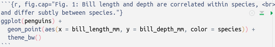
ggplot(penguins) +
  geom_point(aes(x = bill_length_mm, y = bill_depth_mm, color = species)) +
  theme_bw()
#> Warning: Removed 2 rows containing missing values (geom_point).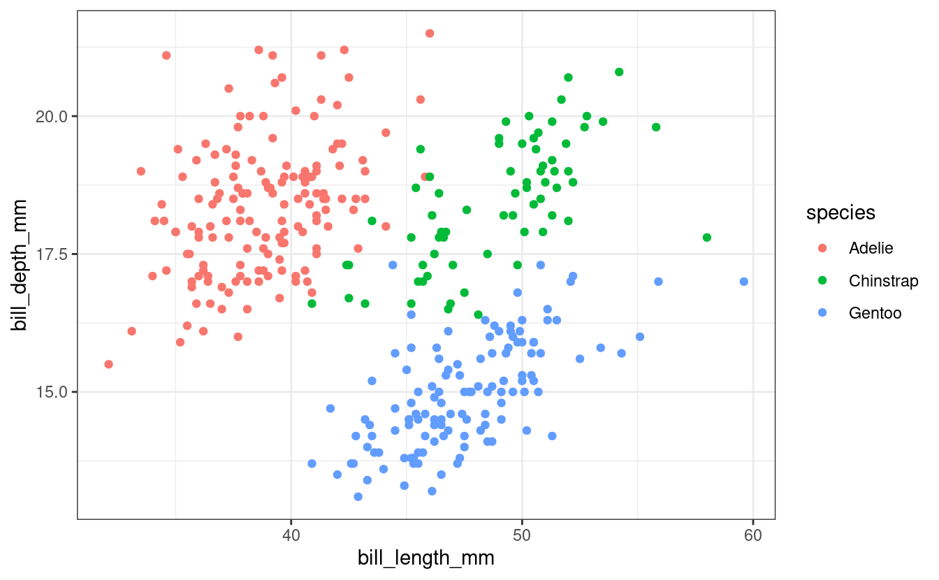
Fig. 1: Bill length and depth are correlated within species,
and differ subtly between species.
We added a caption for the figure using the fig.cap option.
Code chunk options
There are huge number of options, and various options are specific to certain types of code chunks. Just learn the basic structure first, and if you ever wonder “Can I do X to modify the output?” just know that many, many people have wondered that before, and if it makes sense to do it, you can probably do it with options.
Here is an overview of some the most commonly made changes to defaults for code chunk options. This quickly gets confusing, but you’ll get the hang of it after experimenting a bit.
echo=FALSE– Don’t print the code in the output file.eval=FALSE– Don’t run (evaluate) the code.include=FALSE– Run but don’t print the code, nor any of its results.results="hide"– Don’t print the text output of the code.fig.show="hide"– Don’t print figures produced by the code.
Furthermore, you can use message=FALSE and warning=FALSE to suppress any messages (like the output when loading packages) and warnings (like the warning for the penguin figure above), respectively, that R might produce.
For figures, the following options are especially useful:
fig.cap="My caption"– Include a caption.fig.asp=0.6– Aspect ratio.fig.width=6– Width of in inches: same as sizing in regular R code.fig.height=9.6– Height in inches: same as sizing in regular R code.out.width="70%"– Figure width as printed in the document (in%or pixels,px).out.height="500px"– Figure height as printed in the document.
III: The YAML header
YAML (“YAML Ain’t Markup Language”) is a simple format commonly used for configuration files, which allows you to provide key-value pairs such as author: John Doe.
In R Markdown files, it is used as a header which configures certain aspects of the output, especially the formatting. Put another way, the YAML header contains the metadata for the output.
A basic YAML header
Here is an example of a very basic YAML header:
---
author: My name
title: The document's title
output: html_document
---
Note the lines which just contain three dashes, which mark the beginning and the end of the YAML header.
Adding extra options
Often, a value (like html_document) can itself be given key-value pairs to specify additional options – see the example below where we include a Table of Contents (toc) and also set it to “float”:
---
output:
  html_document:
    toc: true
    toc_float: true
---
- Note that indentation in YAML uses two (or four) spaces (no tabs!) per indentation level, and it is sensitive to indentation errors. (Fortunately, RStudio inserts spaces for tabs by default – check/set in
Tools=>Global Options=>Code=>Editing.)
Some options for html_document output
html_document is the most commonly used output format for R Markdown documents, and here are few particularly useful options to customize the output:
code_download: true– Include a button to download the code.code_folding: hide– Usinghideorshowwill enable the folding of code chunks, withhidehiding them by default.toc: true– Include a table of contents (Also:toc_depth: 3sets depth to 3,toc_float: truelets the TOC “float” as you scroll down the document).number_sections: true– Number the section headings.df_print: paged– Get nicely formatted and paged data frame printing (also try:df_print: kable).theme: cerulean– Use a pre-built theme, controlling the overall look and feel of the document. See here for a visual overview.
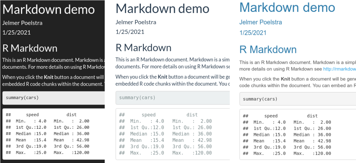
theme options: darkly, flatly, and cerulean.
IV: R Markdown and RStudio
The R Markdown ecosystem of packages is being developed by RStudio, so it should come as no surprise that the RStudio IDE has some nice R Markdown functionality.
Knitting and previewing your document
The process of rendering an R Markdown file into another format, as specified by the YAML header, is called knitting. We already saw the button to knit the current document (keyboard shortcut: Cmd/Ctrl+Shift+K).
If you get preview pop-up windows in RStudio, click the cog wheel icon next to the Knit button, and then select “Preview in Viewer Pane”.
Instead of knitting the entire document, you can also run individual code chunks using the green “play button” (or Cmd/Ctrl+Shift+Enter), or all code chunks up until the current one (button to the left of the play button).
Breakout Room 2
For this exercise, you’ll convert an R Script file into an R Markdown file.
First you’ll download the script file to your working directory (using the code provided below). Then open it in R Studio, copy the contents, and paste the contents into your demo.Rmd file (after the YAML header). Then work through making adjustments, and Knit at various times to check your work.
There are various suggestions (in parentheses) for Markdown formatting throughout the script.
And remember, you need to wrap the actual R code from the script inside R Markdown code chunks.
You’ll also download an example picture. Include this picture in your demo.Rmd file using the Markdown syntax shown above. Then experiment with the various figure options to get it how you want it.
We’ll download the files in a similar way to last week. Execute the following code, either by copying into the console, or by creating a new script file and copying the commands into it, and executing them one by one. To keep things tidy and readable, first we create objects that hold the URLs we’re downloading from:
script_URL <- "https://raw.githubusercontent.com/biodash/biodash.github.io/master/content/codeclub/S02E03_rmarkdown/demo.R"
picture_URL <- "https://raw.githubusercontent.com/biodash/biodash.github.io/master/content/codeclub/S02E03_rmarkdown/picture.jpg"
Then use the download.file() function with two arguments, the remote URL and the local file name (which must be in quotes):
download.file(url = script_URL, destfile = "demo.R")
download.file(url = picture_URL, destfile = "picture.jpg")
You should end up with the two local files showing up in your Files pane.
V: A single source doc, many output formats!
Because of the Pandoc backend, a great feature of R Markdown is that you can output to many formats. So from one source document, or very similar variants, you can create completely different output depending on what you need.
Built-in output formats
The built-in output formats, which can be used with just the rmarkdown package, are listed below. These include HTML, PDF, Word, PowerPoint, and different HTML slide show formats.

Extension output formats
It’s worth highlighting a few of the output formats that can be used with the following packages in the R Markdown ecosystem:
-
distill – An output format geared towards technical content, e.g. with extended support for equations, citations, and footnotes. Can also create websites.
-
rticles – R Markdown templates to format output for specific scientific journals.
-
flexdashboard – Create interactive “dashboards” to present data.
-
bookdown – A book format, the R Markdown book is an example.
-
xaringan – Create fancier presentation slides thanks to a JavaScript library.
Starting to use these and other output formats is often as simple as changing the YAML header:
---
output: distill::distill_article
---
Further resources
-
Free online books by the primary creator of R Markdown and other authors: