Session 14: Writing your own Functions

New To Code Club?

• First, check out the Code Club Computer Setup instructions, which also has some pointers that might be helpful if you’re new to R or RStudio.

• Please open RStudio before Code Club to test things out – if you run into issues, join the Zoom call early and we’ll troubleshoot.

Session Goals

• Learn another way to avoid repetition in your code by creating your own functions.
• Learn the basic template of a function in R.
• Learn to incorporate your own functions into for loops and functionals like lapply() and map().
• Learn all the advantages of using functions instead of copied code blocks.

We’ll be using tibble() and map() from the tidyverse packages, so we need to load that first.

library(tidyverse)

#> ── Attaching packages ─────────────────────────────────────── tidyverse 1.3.0 ──

#> ✔ ggplot2 3.3.2     ✔ purrr   0.3.4
#> ✔ tibble  3.0.4     ✔ dplyr   0.8.5
#> ✔ tidyr   1.0.3     ✔ stringr 1.4.0
#> ✔ readr   1.3.1     ✔ forcats 0.5.0

#> ── Conflicts ────────────────────────────────────────── tidyverse_conflicts() ──
#> ✖ dplyr::filter() masks stats::filter()
#> ✖ dplyr::lag()    masks stats::lag()

Why write functions?

Copying your code is not good

The first motivation for writing a function is when you find yourself cut-and-pasting code blocks with slight alterations each time.

Say we have the following toy tidyverse data frame, where each column is a vector of 10 random numbers from a normal distribution, with mean = 0 and sd = 1 (the defaults for rnorm):

df <- tibble(
  a = rnorm(10),
  b = rnorm(10),
  c = rnorm(10),
  d = rnorm(10)
)

df

#> # A tibble: 10 x 4
#>         a      b       c       d
#>     <dbl>  <dbl>   <dbl>   <dbl>
#>  1  0.388  0.736  2.26   -0.302 
#>  2  1.19  -0.131 -2.17   -0.0537
#>  3  0.971  0.919  0.0329 -0.227 
#>  4 -0.147 -1.43   1.15   -2.09  
#>  5  1.87   0.566 -0.935   0.601 
#>  6 -1.07   0.941  1.56   -0.413 
#>  7  1.22   0.637  1.62    0.976 
#>  8 -0.142  1.02   1.98    1.22  
#>  9 -2.02   0.499 -1.93   -0.0917
#> 10  0.177  0.347  1.79    1.55

In previous Code Clubs we’ve seen how you can apply a built-in function like median to each column using a for loop or lapply. But say we wanted to do something a bit fancier that is not part of core R. For example, we can normalize the values in a column so they range from 0 to 1 using the following code block:

(df$a - min(df$a)) / (max(df$a) - min(df$a))

#>  [1] 0.6193844 0.8252053 0.7693140 0.4817556 1.0000000 0.2453463 0.8345409
#>  [8] 0.4828838 0.0000000 0.5650749

This code is a literal translation of the mathematical formula for normalization:

$$z_{i} = \frac{x_{i} - min(x)}{max(x)-min(x)}$$ OK, so how can we do this for each column? Here is a first attempt:

df$a <- (df$a - min(df$a)) / (max(df$a) - min(df$a))
df$b <- (df$b - min(df$a)) / (max(df$b) - min(df$b))
df$c <- (df$c - min(df$c)) / (max(df$c) - min(df$c))
df$d <- (df$d - min(df$d)) / (max(df$d) - min(df$d))

df

#> # A tibble: 10 x 4
#>        a       b      c     d
#>    <dbl>   <dbl>  <dbl> <dbl>
#>  1 0.619  0.301  1      0.491
#>  2 0.825 -0.0535 0      0.559
#>  3 0.769  0.376  0.497  0.512
#>  4 0.482 -0.582  0.749  0    
#>  5 1      0.231  0.278  0.739
#>  6 0.245  0.384  0.843  0.461
#>  7 0.835  0.260  0.855  0.842
#>  8 0.483  0.418  0.938  0.910
#>  9 0      0.204  0.0532 0.549
#> 10 0.565  0.142  0.895  1

This works, but it caused me mental anguish to type it out. Even with cut and paste! All those manual textual substitutions!! And manual data entry is prone to mistakes, especially repetitive tasks like this. And say you had 1,000 columns…

And it didn’t work!! Honestly, I swear that mistake was totally real: I didn’t notice it until I looked at the output. Can you spot the mistake?

It turns out R has a range function that returns the minimum and maximum of a vector, which somewhat simplifies the coding:

range(df$a)

The result is a vector something like c(-1.2129504, 2.1011248) (it varies run to run, since the columns values are random) which we can index, and so we only do the min/max computation once for each column, instead of three times, so we get the following block of code for each column:

rng <- range(df$a)
(df$a - rng[1]) / (rng[2] - rng[1])

Does this help?

rng <- range(df$a)
df$a <- (df$a - rng[1]) / (rng[2] - rng[1])

rng <- range(df$b)
df$b <- (df$b - rng[1]) / (rng[2] - rng[1])

rng <- range(df$c)
df$c <- (df$c - rng[1]) / (rng[2] - rng[1])

rng <- range(df$d)
df$d <- (df$d - rng[1]) / (rng[2] - rng[1])

Still pretty horrible, and arguably worse since we add a line for each column.

How can we distill this into a function to avoid all that repetition?

Encapsulation of code in a function

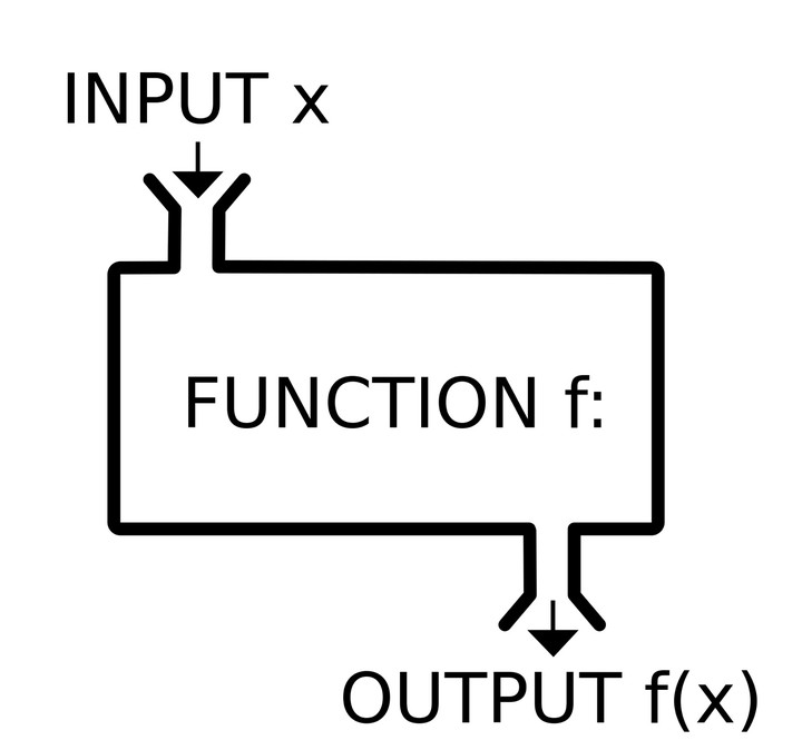
The secret to function writing is abstracting the constant from the variable. (Using the range function does throw into sharper relief what is constant and what is varying at least.) The constant part is the body of the function: the template or boiler-plate you use over and over again. The variable parts are the arguments of the function. We also need to give the function a name, so we can call it and reuse it. The template for a function is then:

name <- function(arg1, arg2...) {
  <body> # do something with arg1, arg2
}

The arguments go inside (...). The body is the block of code you want to reuse, and it’s contained in curly brackets {...}.

Here’s what it looks like in this case:

normalize <- function(x) {
  rng <- range(x)
  (x - rng[1]) / (rng[2] - rng[1])
}

Pretty cool, right? Here normalize is the descriptive name we give the function.

We assign the function to the name using <- just like any other value. This means that now normalize is a function object, just like you create vector objects, or list or data frame objects, when you assigned them to names. Notice too that in RStudio they appear in the Global Environment in a special section, and clicking on them shows the code. This means that if you have a large file of code with many functions defined, you don’t have to go back searching for the function definition in the code itself.

x is the argument of the function. In the current case this is a data frame column vector, but we can potentially use this function on any vector, so let’s not be too specific. The more generally you can write your function, the more useful it will be.

test_vec <- c(3, 7, pi, 8.657, 80)
normalize(test_vec)

#> [1] 0.000000000 0.051948052 0.001838866 0.073467532 1.000000000

When we call the function, the value we use in the function call is assigned to x and is passed in to the body of the function. So if we call the function on the first column, it gets passed in to the body, and returns the result:

df <- tibble(a = rnorm(10))
normalize(df$a)

#>  [1] 0.8726863 1.0000000 0.8764474 0.5618469 0.6111361 0.4147958 0.2889830
#>  [8] 0.2683500 0.7181709 0.0000000

A couple of things to note:

• Including that extra line rng <- range(x) is no longer a problem, since we just type it once. If you are typing things out over and over you might prefer brevity. When you write a function, you should prefer clarity. It’s good practice to break the the function down into logical steps, and name them properly. It’s much easier for others to ‘read’ your function, and much easier for you when you come back to it in a couple of years. This is the principle of making your code ‘self-annotated’.

• Functions should be simple, clear, and do one thing well. You create programs by combining simple functions in a modular manner.

• There’s something very important but rather subtle about this use of the argument. As noted in CodeClub 12, once a for loop completes, the variable you’re using keeps the value it had at the last iteration of the loop, which persists in the global environment. Below we’ll compare that behavior to what happens with the function’s x argument.

Our original horrible code can now be rewritten as:

df$a <- normalize(df$a)
df$b <- normalize(df$b)
df$c <- normalize(df$c)
df$d <- normalize(df$d)

Which is an improvement, but the real power comes from the fact that we can use our new function in for loops and apply statements. Here is the data from the previous couple of Clubs:

dists_Mar4 <- c(17, 93, 56, 19, 175, 40, 69, 267, 4, 91)
dists_Mar5 <- c(87, 143, 103, 223, 106, 18, 87, 72, 59, 5)
dist_df <- data.frame(dists_Mar4, dists_Mar5)

Let’s first sanity check that our new function behaves sensibly on these vectors:

normalize(dists_Mar4)

#>  [1] 0.04942966 0.33840304 0.19771863 0.05703422 0.65019011 0.13688213
#>  [7] 0.24714829 1.00000000 0.00000000 0.33079848

normalize(dists_Mar5) 

#>  [1] 0.37614679 0.63302752 0.44954128 1.00000000 0.46330275 0.05963303
#>  [7] 0.37614679 0.30733945 0.24770642 0.00000000

And while we’re here, let’s circle back to the assignment of the x argument outside and inside the function. Below we first assign a value to x outside the function; pass in a value to x inside the function; then reevaluate x outside the function call, to see what happens:

x = pi
x

#> [1] 3.141593

normalize(dists_Mar5)             # inside the function, x <- dists_Mar5

#>  [1] 0.37614679 0.63302752 0.44954128 1.00000000 0.46330275 0.05963303
#>  [7] 0.37614679 0.30733945 0.24770642 0.00000000

x

#> [1] 3.141593

Whatever value x has outside the function does not affect, and is not affected by, the value of x inside the function. In computer science terms we say the variable(s) used inside the function are local to the function. They are freshly minted inside it, and safely destroyed before you leave it. So there is no chance of weird or unexpected conflicts with whatever variable values are set outside. In contrast, the variable in the for loop is global. It ‘leaks out’ from where you actually used it, with perhaps unforeseen consequences. This is extremely important when you start embedding your own functions in larger programs.

Default values for arguments

In R, we can assign a default value for an argument using = assignment. This means the argument will be called automatically, but can be overridden if explicitly called. First we create a function in the usual way:

variable_power <- function(x, p){  
  x**p               # raises x to the power p
}

variable_power(2, 3)

#> [1] 8

And now we create a version with a default value for the power:

variable_power_2 <- function(x, p = 2){
  x**p
}

variable_power_2(2)

#> [1] 4

variable_power_2(2, 3)

#> [1] 8

Functions in for loops

Here is how we can use our new function in a for loop over a data frame. In our previous examples of for loops median was a summary statistic and we return a single value for each column, so we created an empty vector of the desired length to hold the values for each column. Here we want to modify the original data frame with the same dimensions and column names. The following code copies the original data frame (so we don’t destroy it) and then modifies the copy ‘in place’:

dist_df_norm <- dist_df
for (column_number in 1:ncol(dist_df)){
  dist_df_norm[[column_number]] <- normalize(dist_df[[column_number]])
}
dist_df_norm

#>    dists_Mar4 dists_Mar5
#> 1  0.04942966 0.37614679
#> 2  0.33840304 0.63302752
#> 3  0.19771863 0.44954128
#> 4  0.05703422 1.00000000
#> 5  0.65019011 0.46330275
#> 6  0.13688213 0.05963303
#> 7  0.24714829 0.37614679
#> 8  1.00000000 0.30733945
#> 9  0.00000000 0.24770642
#> 10 0.33079848 0.00000000

Copying an entire data frame could take a lot of time. So we can also create an empty data frame (of the same dimensions) and populate it:

empty_vec <- vector(length = nrow(dist_df))
dist_df_norm_2 <- tibble(norm_Mar4 = empty_vec, norm_Mar5 = empty_vec)

for (column_number in 1:ncol(dist_df)){
  dist_df_norm_2[[column_number]] <- normalize(dist_df[[column_number]])
}
dist_df_norm_2

#> # A tibble: 10 x 2
#>    norm_Mar4 norm_Mar5
#>        <dbl>     <dbl>
#>  1    0.0494    0.376 
#>  2    0.338     0.633 
#>  3    0.198     0.450 
#>  4    0.0570    1     
#>  5    0.650     0.463 
#>  6    0.137     0.0596
#>  7    0.247     0.376 
#>  8    1         0.307 
#>  9    0         0.248 
#> 10    0.331     0

By writing our own function, we’ve effectively extended what R can do. And this is all that packages are: libraries of new functions that extend the capabilities of base R. In fact, if there are functions you design for your particular subject area and find yourself using all the time, you can make your own package and load it, and all your favorite functions will be right there (but that’s for another day…)

Functional programming with your own functions

We saw above that you assign the function object to a name, just as you would a vector, list or data frame. In R, functions are ‘first class citizens’, which means you can pass them as arguments to another function. This is a very powerful idea, and part of the program of functional programming (we introduced this idea in Session 13):

In functional programming, functions are treated as first-class citizens, meaning that they can be bound to names…, passed as arguments, and returned from other functions, just as any other data type can.

Functions that take other functions as arguments are sometimes referred to as functionals.

In the previous session we showed how to use built-in functions like median as arguments to functionals. The functions you write yourself can also be used in exactly the same way.

lapply()

We introduced this functional in Session 13: it always returns a list:

lapply_norm <- lapply(dist_df, normalize)
lapply_norm

#> $dists_Mar4
#>  [1] 0.04942966 0.33840304 0.19771863 0.05703422 0.65019011 0.13688213
#>  [7] 0.24714829 1.00000000 0.00000000 0.33079848
#> 
#> $dists_Mar5
#>  [1] 0.37614679 0.63302752 0.44954128 1.00000000 0.46330275 0.05963303
#>  [7] 0.37614679 0.30733945 0.24770642 0.00000000

typeof(lapply_norm)

#> [1] "list"

str(lapply_norm)

#> List of 2
#>  $ dists_Mar4: num [1:10] 0.0494 0.3384 0.1977 0.057 0.6502 ...
#>  $ dists_Mar5: num [1:10] 0.376 0.633 0.45 1 0.463 ...

sapply() attempts to simplify the outputs. Here both lists are of type num, and the same length, so in this case R simplifies to a matrix data structure with a single type:

sapply_norm <- sapply(dist_df, normalize)
sapply_norm

#>       dists_Mar4 dists_Mar5
#>  [1,] 0.04942966 0.37614679
#>  [2,] 0.33840304 0.63302752
#>  [3,] 0.19771863 0.44954128
#>  [4,] 0.05703422 1.00000000
#>  [5,] 0.65019011 0.46330275
#>  [6,] 0.13688213 0.05963303
#>  [7,] 0.24714829 0.37614679
#>  [8,] 1.00000000 0.30733945
#>  [9,] 0.00000000 0.24770642
#> [10,] 0.33079848 0.00000000

typeof(sapply_norm)

#> [1] "double"

dim(sapply_norm)

#> [1] 10  2

str(sapply_norm)

#>  num [1:10, 1:2] 0.0494 0.3384 0.1977 0.057 0.6502 ...
#>  - attr(*, "dimnames")=List of 2
#>   ..$ : NULL
#>   ..$ : chr [1:2] "dists_Mar4" "dists_Mar5"

lapply() yields a named list, sapply() yields a named matrix.

purrr::map()

The functional map() from the purrr package behaves the same as lapply(), it always returns a list (purrr is automatically loaded as part of the tidyverse):

map_norm <- map(dist_df, normalize)
map_norm

#> $dists_Mar4
#>  [1] 0.04942966 0.33840304 0.19771863 0.05703422 0.65019011 0.13688213
#>  [7] 0.24714829 1.00000000 0.00000000 0.33079848
#> 
#> $dists_Mar5
#>  [1] 0.37614679 0.63302752 0.44954128 1.00000000 0.46330275 0.05963303
#>  [7] 0.37614679 0.30733945 0.24770642 0.00000000

typeof(map_norm)

#> [1] "list"

str(map_norm)

#> List of 2
#>  $ dists_Mar4: num [1:10] 0.0494 0.3384 0.1977 0.057 0.6502 ...
#>  $ dists_Mar5: num [1:10] 0.376 0.633 0.45 1 0.463 ...

Notice another advantage of both lapply() and map(): we don’t need to explicitly preallocate any kind of data structure to collect the results. The allocation is done behind the scenes as part of the implementation of lapply() and map(), which makes sure they run efficiently. In fact, R implements these functionals as a for loop behind the scenes, and in map() that for loop is implemented in C, so it optimizes performance.

If we want the output to be a data frame to match the input, we can simply coerce it:

map_norm_df <- map(dist_df, normalize) %>% 
  as_tibble
str(map_norm_df)

#> tibble [10 × 2] (S3: tbl_df/tbl/data.frame)
#>  $ dists_Mar4: num [1:10] 0.0494 0.3384 0.1977 0.057 0.6502 ...
#>  $ dists_Mar5: num [1:10] 0.376 0.633 0.45 1 0.463 ...

Advantages of using functions

Functions:

• avoid duplication, save time
• avoid coding errors in repetitive code
• localize variables, avoiding unexpected assignment surprises
• let you modify code in a single place, not multiple places
• lets you reuse code, since a single function can often be used on multiple inputs (vectors, lists and data frames), and can be imported from a package, instead of copy and paste.

Breakout rooms

Exercise 1

cv <- function(v){
  sd(v)/mean(v)
}

cv(1:200)

#> [1] 0.5759123

Exercise 2

equalish <- function(a, b, epsilon = 0.000001){
  abs(a - b) < epsilon
}

equalish(4.0, 4.01)

#> [1] FALSE

equalish(4.0, 4.000000001)

#> [1] TRUE

v1 <- c(4.000000001, 2)
v2 <- c(4.0, 7)

equalish(v1, v2)

#> [1]  TRUE FALSE

equalish(v1, v2, 0.000000000000001)

#> [1] FALSE FALSE

Exercise 3

@SIM:1:FCX:1:15:6329:1045 1:N:0:2
TCGCACTCAACGCCCTGCATATGACAAGACAGAATC
+
<>;##=><9=AAAAAAAAAA9#:<#<;<<<????#=

utf8ToInt("!")

#> [1] 33

phred_score <- function(character){
  utf8ToInt(character) - 33
}

phred_score("<>;##=><9=AAAAAAAAAA9#:<#<;<<<????#=")

#>  [1] 27 29 26  2  2 28 29 27 24 28 32 32 32 32 32 32 32 32 32 32 24  2 25 27  2
#> [26] 27 26 27 27 27 30 30 30 30  2 28