Session 12: Vectorization and loops in R
Need for repeat.
 Artwork by @allison_horst
Setup
New to Code Club?
-
If you didn’t already do this, please follow the Code Club Computer Setup instructions, which also have pointers for if you’re new to R or RStudio.
-
If you’re able to do so, please open RStudio a bit before Code Club starts – and in case you run into issues, please join the Zoom call early and we’ll help you troubleshoot.
Session goals
Today, you will learn:
- That you should avoid copying your code.
- What different strategies for iteration exist in R.
- What vectorization is and how to make use of it.
- How to write a
forloop. - Best practices when using
forloops. - When you should (not) use
forloops. - Bonus:
ifstatements.
Introduction
Don’t Repeat Yourself
Sometimes, you have a block of code and you need to repeat the operations in that code almost exactly. For instance, you may want to rerun a statistical model with different parameter values, rerun an analysis for a different batch of samples, or extract the same information for many different genes.
Your first instinct may be to copy-and-paste the block of code, and make the necessary slight adjustments in the pasted block. However, iterating and writing your own functions are strategies that are clearer, less error-prone, and more flexible (and these two can also be combined). When the number of repeats are high, iteration is needed. When the code that needs to be repeated is more than a line or two, writing your own functions becomes useful.
Iteration
Loops are the most universal iteration tool and the one we will focus on today. However, R has “functional programming” iteration methods that are less verbose and that can also be quicker to execute. These are the apply family of functions, and a more recent tidyverse approach implemented in the purrr package: we will learn more about those in the two upcoming Code Club sessions.
Loops are still a very good place to start using iteration because they make the iteration explicit and are therefore more intuitive than functional alternatives. In addition, they can easily accommodate longer blocks of code without the need to also write your own function.
Today, we will talk about the most common type of loop: the for loops. (Other types of loops in R are while loops and repeat loops. Related to loops are if statements, see the bonus exercise for some basics.)
But first…
Before we tackle loops we should take a step back and explore vectorization a bit more, which was briefly introduced by Michael in Code Club session 9. Besides functional programming methods, vectorization is the other reason that loops are not as widely used in R as in other programming languages.
I: Vectorization
Let’s say we have a vector (i.e., a collection of values) that consists of distances in miles:
dists_miles <- c(24, 81, 48, 29, 177, 175, 20, 11, 62, 156)Of course, we can’t science with miles, so we’ll have to convert these distances to kilometers by multiplying each value in the vector by 1.61. You may or may not know that this can be done really easily in R:
dists_km <- dists_miles * 1.61
dists_km
#>  [1]  38.64 130.41  77.28  46.69 284.97 281.75  32.20  17.71  99.82 251.16
What is happening here is called a vectorized operation: 1.61 is automatically recycled as many times as needed to be multiplied with each individual value in the dist_miles vector. This is a pretty unique and very useful feature of R!
In many other languages, we would need a loop or a similar construct to iterate over each value in the vector and multiply by 1.61. In fact, under the hood, R also uses a loop to do this! So does it even make a difference? Yes – the advantages of using vectorization in R are:
-
You don’t have to write the loop, saving you a fair bit of typing and making the code clearer.
-
The under-the-hood-loop is being executed much faster than a loop that you would write. This is because it is written in
C/C++code which only has to be called once (instead of at least as many times as there are iterations in our loop).
Other vectorization patterns
Above, we saw an example of multiplying a vector by a single number. We can also use vectorized operations when both objects contain multiple items. For instance, say we have a vector with corresponding values for two dates:
dists_Mar4 <- c(17, 93, 56, 19, 175, 40, 69, 267, 4, 91)
dists_Mar5 <- c(87, 143, 103, 223, 106, 18, 87, 72, 59, 5)
To get the sum of these values at each position (index) of the two vectors (17 + 87, 93 + 143, etc.), we can simply do the following:
dists_Mar4 + dists_Mar5
#> [1] 104 236 159 242 281 58 156 339 63 96This also works for columns of a data frame, which we can extract using the dataframe_name$column_name notation (see Code Club session 9’s section on data frames, and the Base R data frame indexing summary below). Let’s say we wanted the mean distance this time:
dist_df <- data.frame(dists_Mar4, dists_Mar5)

dist_df$dists_mean = (dist_df$dists_Mar4 + dist_df$dists_Mar5) / 2
head(dist_df)
#>   dists_Mar4 dists_Mar5 dists_mean
#> 1         17         87       52.0
#> 2         93        143      118.0
#> 3         56        103       79.5
#> 4         19        223      121.0
#> 5        175        106      140.5
#> 6         40         18       29.0
Vectorization with matrices
Furthermore, we can also perform vectorized operations on entire matrices. With the following matrix:
## We use the "sample" function to get 25 random values between 1 and a 100,
## and put those in a 5*5 matrix:
mat <- matrix(sample(1:100, 25), nrow = 5, ncol = 5)
mat
#>      [,1] [,2] [,3] [,4] [,5]
#> [1,]    2   55    8   28   24
#> [2,]   81   30   99   33   12
#> [3,]   22   67   41   54    6
#> [4,]   48   84   42   35  100
#> [5,]   57   47   93   10   31
…we could multiple all values by 10 or get the square of each value simply as follows:
mat_more <- mat * 10
mat_more
#>      [,1] [,2] [,3] [,4] [,5]
#> [1,]   20  550   80  280  240
#> [2,]  810  300  990  330  120
#> [3,]  220  670  410  540   60
#> [4,]  480  840  420  350 1000
#> [5,]  570  470  930  100  310

mat_squared <- mat * mat
mat_squared
#>      [,1] [,2] [,3] [,4]  [,5]
#> [1,]    4 3025   64  784   576
#> [2,] 6561  900 9801 1089   144
#> [3,]  484 4489 1681 2916    36
#> [4,] 2304 7056 1764 1225 10000
#> [5,] 3249 2209 8649  100   961
Vectorization with indices
We can also use vectorized solutions when we want to operate only on elements that satisfy a certain condition.
Let’s say we consider any distance in one of our vectors that is below 50 to be insufficient, and we want to turn those values into negatives (a little harsh maybe, but we go with it).
To do so, we make use of R’s ability to index a vector with a logical vector:
## "not_far_enough" will be a vector of logicals:
not_far_enough <- dists_Mar4 < 50
not_far_enough
#>  [1]  TRUE FALSE FALSE  TRUE FALSE  TRUE FALSE FALSE  TRUE FALSE

## When we index the original vector with a logical vector,
## we get only those values for which "not_far_enough" is TRUE:
dists_Mar4[not_far_enough]
#> [1] 17 19 40  4
With the following syntax, we can replace just those low distances in our original vector:
dists_Mar4[not_far_enough] <- dists_Mar4[not_far_enough] * -1
dists_Mar4
#> [1] -17 93 56 -19 175 -40 69 267 -4 91II: For loops
While it is important to use vectorization whenever possible, it can only be applied to a specific set of problems. A more universal solution when you need to repeat operations is the for loop. for loops iterate over a collection of values, allowing you to perform one or more actions for each value in the collection.
The basic syntax is as follows:
for (variable_name in collection_name) {
  #...do things for each item (variable_name) in the collection, one at a time...
}
On the first line, you initialize the for loop, telling it to assign each item in the collection to a variable (here, variable_name) one at a time.
The variable name is arbitrary, and the collection is whatever you want to loop over. However, for, the parentheses (), in, and the curly braces {} are all fixed elements of for loops. A simple example will help to understand the synax:
## A loop to print negated values:
for (one_number in c(1, 2, 3, 4)) {  # We iterate over 1, 2, 3, 4
  print(one_number * -1)             # Multiply each number by -1
}
#> [1] -1
#> [1] -2
#> [1] -3
#> [1] -4
Note that we don’t have to use the variable that we are looping over: we could also use a for loop as a roundabout way to simply repeat something as many times as there are values in our collection:
for (dummy in c(1, 2, 3, 4)) {
  print("Yes!")                     # Print "Yes!" in each of our four iterations
}
#> [1] "Yes!"
#> [1] "Yes!"
#> [1] "Yes!"
#> [1] "Yes!"
As mentioned, the variable name that we assign is arbitrary: we could use anything, as long as we reference it with the same name inside the loop:
## Example 1 with a different variable name: "positive_number"
for (positive_number in c(1, 2, 3, 4)) {
  print(positive_number * -1)
}
#> [1] -1
#> [1] -2
#> [1] -3
#> [1] -4

## Example 2 with a different variable name: "i"
for (i in c(1, 2, 3, 4)) {
  print(i * -1)
}
#> [1] -1
#> [1] -2
#> [1] -3
#> [1] -4
Note that the variable as it was last assigned in the loop does persist in your environment:
i
#> [1] 4
The curly braces are not strictly necessary for one-liners like this:
for (i in 1:4) print(i * -1)
#> [1] -1
#> [1] -2
#> [1] -3
#> [1] -4
for loop output
Note that we need the print() function to print anything to screen – nothing will be printed if we omit this:
for (i in 1:4) {
  i * -1
}
Similarly, if we want the output to be saved in an object of some kind, we need to explicitly make an assignment in each iteration of the loop. This is where we need to start paying attention to the design of our loop. Unless computational speed is of no concern at all, you should avoid growing an object in each iteration of the loop.
For example, you might be inclined to do the following if you wanted to compute the median of each column in a data frame:
## We initialize a vector in which we collect the column medians:
column_medians <- vector()

for (column_number in 1:ncol(dist_df)) {

  ## We extract one column using "dataframe_name[[column_number]]":
  column_median <- median(dist_df[[column_number]])

  ## We add the single-column median to our vector of medians:
  column_medians <- c(column_medians, column_median)
}

column_medians
#> [1] 62.50 87.00 78.75
Similarly, you may be tempted to add a column (with cbind()) or a row (with rbind()) to a data frame in each iteration of the loop. However, the problem with these approaches is that R has to create an entirely new object in each iteration of the loop, because the object’s memory requirements keep increasing.
Instead, you’ll want to give the final vector (here, column_medians) the appropriate size before you start the loop:
column_medians <- vector(length = ncol(dist_df))

for (column_number in 1:ncol(dist_df)) {
  column_median <- median(dist_df[[column_number]])
  column_medians[column_number] <- column_median
}
Note that for very small problems, such as the example above, there will not be a noticeable difference in computation time between pre-assigning a properly sized object versus growing an object inside the loop. However, it is still good to get into the habit of pre-assigning an object of the right size.
Summary guidelines (when speed is an issue)
- Don’t use a loop when you can instead use vectorized operations.
- Don’t grow objects inside the loop. Instead, pre-assign an object large enough to contain all output of the loop and fill it in inside the loop.
- When you write a loop, avoid doing things inside the loop that don’t need to be repeated.
Learning about how to create your own functions and/or to use functional programming techniques like purrr and the apply family of functions (upcoming Code Club sessions!) will likely reduce your reliance on loops. For instance, as we’ll see next week, computing the median of each column in a data frame can be done much more succinctly with apply().
Even for more experienced users, loops remain a more viable option when longer blocks of code need to be repeated: we will practice with that in the exercises.
Breakout rooms!
For the exercises, you can download an R Markdown file with some code to get set up (I recommend coding in that document to get a nice overview of the maps that you will make):
dir.create('S12')
todays_rmd <- 'https://raw.githubusercontent.com/biodash/biodash.github.io/master/content/codeclub/12_loops/exercises.Rmd'
download.file(url = todays_rmd, destfile = 'S12/exercises.Rmd')
The following code is already in your R Markdown file, which will download and read the bird dataset and the necessary packages:
## Download the file with bird data:
birds_url <- 'https://raw.githubusercontent.com/biodash/biodash.github.io/master/assets/data/birds/backyard-birds_sample_error.tsv'
birds_file <- 'backyard-birds_sample_error.tsv'
download.file(url = birds_url, destfile = birds_file)
## Load the tidyverse:
library(tidyverse)
## Read the file with bird data:
birds <- read_tsv(birds_file)
## Load the maps package and get the state map:
# install.packages('maps') # first install if necessary
library(maps)
states <- map_data("state")Last week, we learned about making maps. If you attended one of the first few Code Club sessions, you’ll recall our Great Backyard Birdcount data set. Here, we’ll use a country-wide random subset of this data (the full file is over 4 GB) to see where Carolina Chickadees were seen:
## With this line, we select only the rows where the column "species_en"
## (English species name) equals "Carolina Chickadee",
## i.e. we are getting just the records for the Carolina Chickadee:
caro_chickadee <- birds[birds$species_en == 'Carolina Chickadee', ]

## Or in tidyverse-speak:
# caro_chickadee <- birds %>% filter(species_en == 'Carolina Chickadee')

# Next, we create a map much like we did last week:
ggplot(data = states,                               # Use "states" for underlying map
       mapping = aes(x = long, y = lat, group = group)) +
  geom_polygon(color = "black", fill = "white") +   # Black state outlines, white fill
  geom_point(data = caro_chickadee,                 # Plot points from bird data set
             aes(x = long, y = lat, group = NULL),
             color = "green4", alpha = 0.5) +       # Green points, somewhat transparent
  coord_fixed(1.3) +                                # Fix projection
  labs(title = 'Carolina Chickadee')
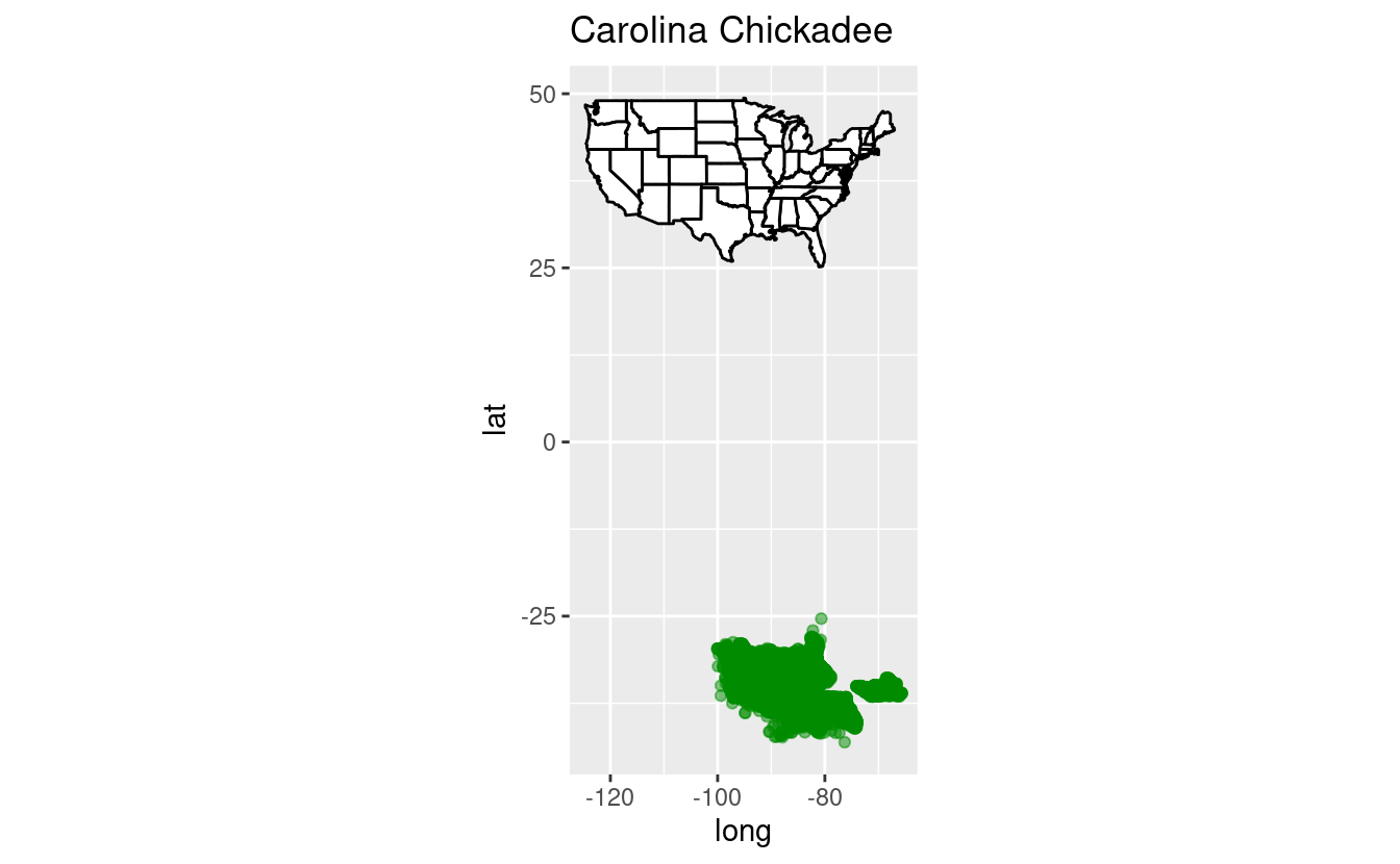
Uh-oh! Something appears to have gone wrong. In the first exercise, you’ll use vectorization to fix the coordinates in the bird data set.
In the second exercise, you’ll use a loop to quickly produce similar plots for several other species.
Exercise 1: Vectorization
Try to fix the coordinates using vectorized operations, and recreate the map to see if it worked.
- Start with the latitude, which is wrong for all points.
Hints (click here)
-
You’ll need to modify the
caro_chickadeedata frame, while you can keep the plotting code exactly the same. -
Simply prepending the latitude column with a minus sign (
-) will negate the values. -
Equivalent base R ways to refer to the column with latitudes are
caro_chickadee$latandcaro_chickadee[['lat']].
Solution (click here)
First we fix the latitude, which was simply negated:
caro_chickadee$lat <- -caro_chickadee$lat

## Or equivalently:
# caro_chickadee[['lat']] <- -caro_chickadee[['lat']]

## Or a tidyverse way of doing this:
# caro_chickadee <- caro_chickadee %>% mutate(lat = -lat)
Create the first map with the same code as the example:
ggplot(data = states,
       mapping = aes(x = long, y = lat, group = group)) +
  geom_polygon(color = "black", fill = "white") +
  geom_point(data = caro_chickadee,
             aes(x = long, y = lat, group = NULL),
             color = "green4", alpha = 0.5) +
  coord_fixed(1.3) +
  labs(title = 'Carolina Chickadee')

- Once you have fixed the latitude, you should notice that for one state, there is a problem with the longitude (the offset is 10 decimal degrees).
Hints (click here)
-
The displaced state is North Carolina.
-
The state of each sighting is in the
stateProvincecolumn, and North Carolina’s name is simply “North Carolina” in that column. -
It may help to first create a logical vector indicating whether for each row in the
caro_chickadeedata frame,stateProvinceforequals “North Carolina”. -
Your final map will look nicer if you get rid of the plotting canvas by adding
+ theme_void()to the code for the plot.
Solution (click here)
It turns out that North Carolina’s chickadees are above the Atlantic. Let’s perform a rescue operation by fixing the longitudes, which are offset by 10 degrees, just for North Carolina:
## Get a vector of logicals, indicating which rows are from North Carolina:
NC_rows <- caro_chickadee$stateProvince == "North Carolina"

## Only for North Carolina rows, change the longitude:
caro_chickadee$long[NC_rows] <- caro_chickadee$long[NC_rows] - 10

## Or with ifelse in one line:
# caro_chickadee$long <- ifelse(caro_chickadee$stateProvince == "North Carolina",
#                               caro_chickadee$long - 10,
#                               caro_chickadee$long)

## Or with mutate and ifelse:
# caro_chickadee %>%
#   mutate(long = ifelse(stateProvince == "North Carolina", long - 10, long))
And we create the final map:
ggplot(data = states,
       mapping = aes(x = long, y = lat, group = group)) +
  geom_polygon(color = "black", fill = "white") +
  geom_point(data = caro_chickadee,
             aes(x = long, y = lat, group = NULL),
             color = "green4", alpha = 0.5) +
  coord_fixed(1.3) +
  labs(title = 'Carolina Chickadee') +
  theme_void()
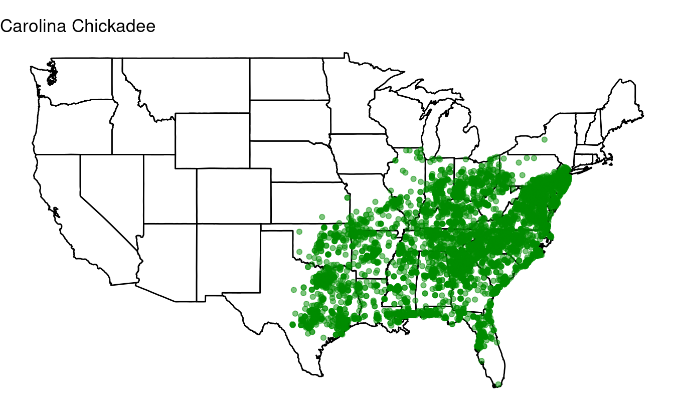
Nice!
Exercise 2: for loops
Find the 10 most commonly observed bird species in the data set, and save their English names (found in the species_en column) in a vector.
Feel free to check out the solution if you’re not sure how, because the focus here is on the next step: trying to create a loop.
Solution (click here)
top10 <- birds %>%
count(species_en, sort = TRUE) %>% # Produces a sorted count table for "species_en"
pull(species_en) %>% # Extracts the "species_en" column
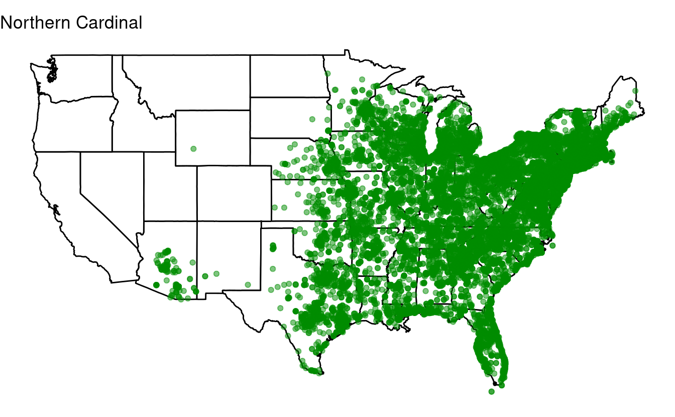
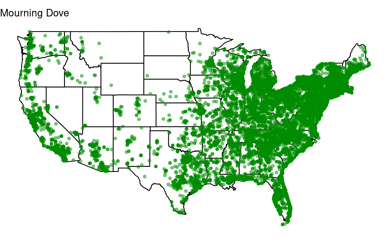
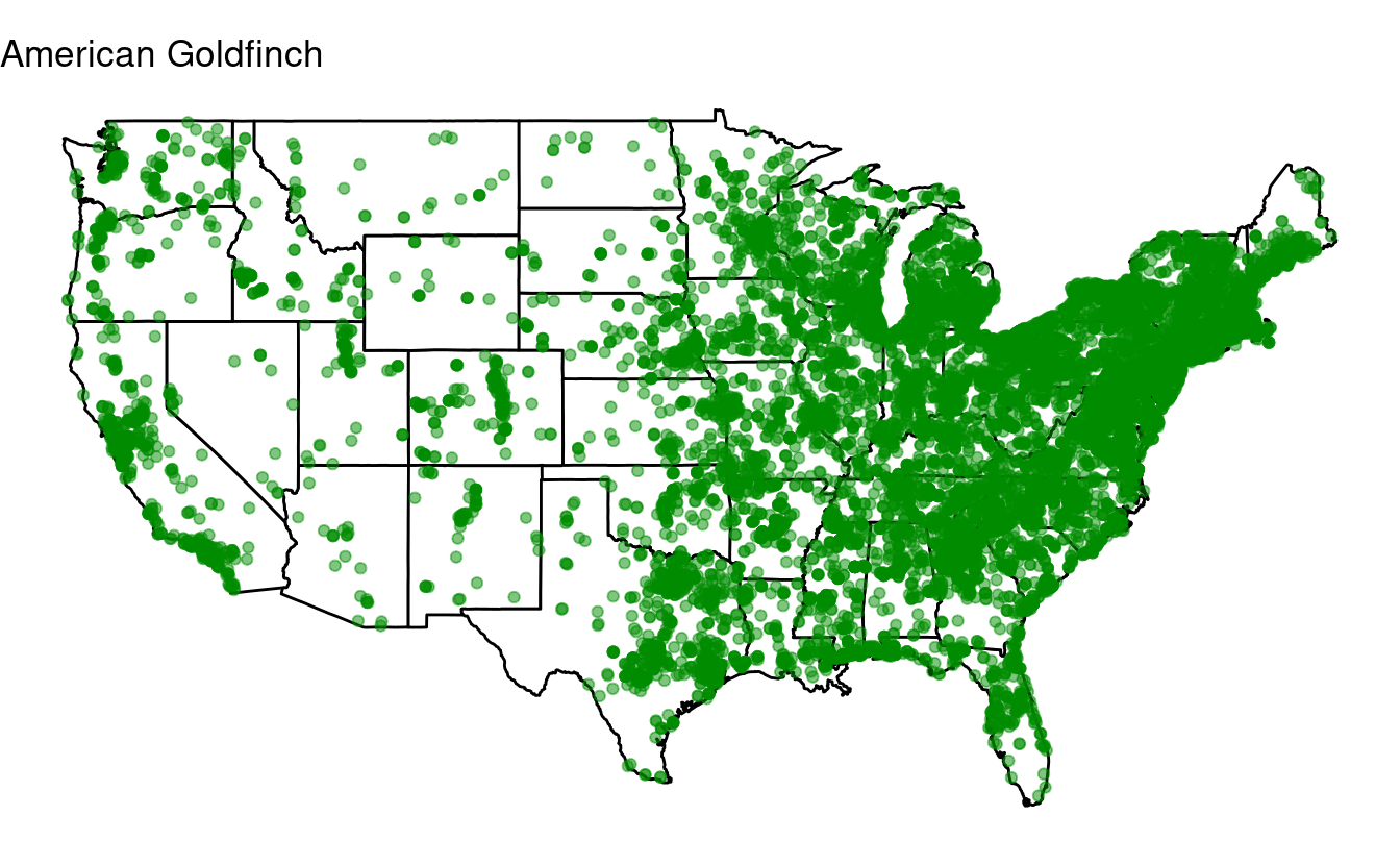
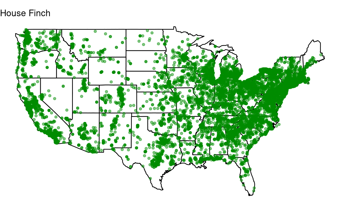
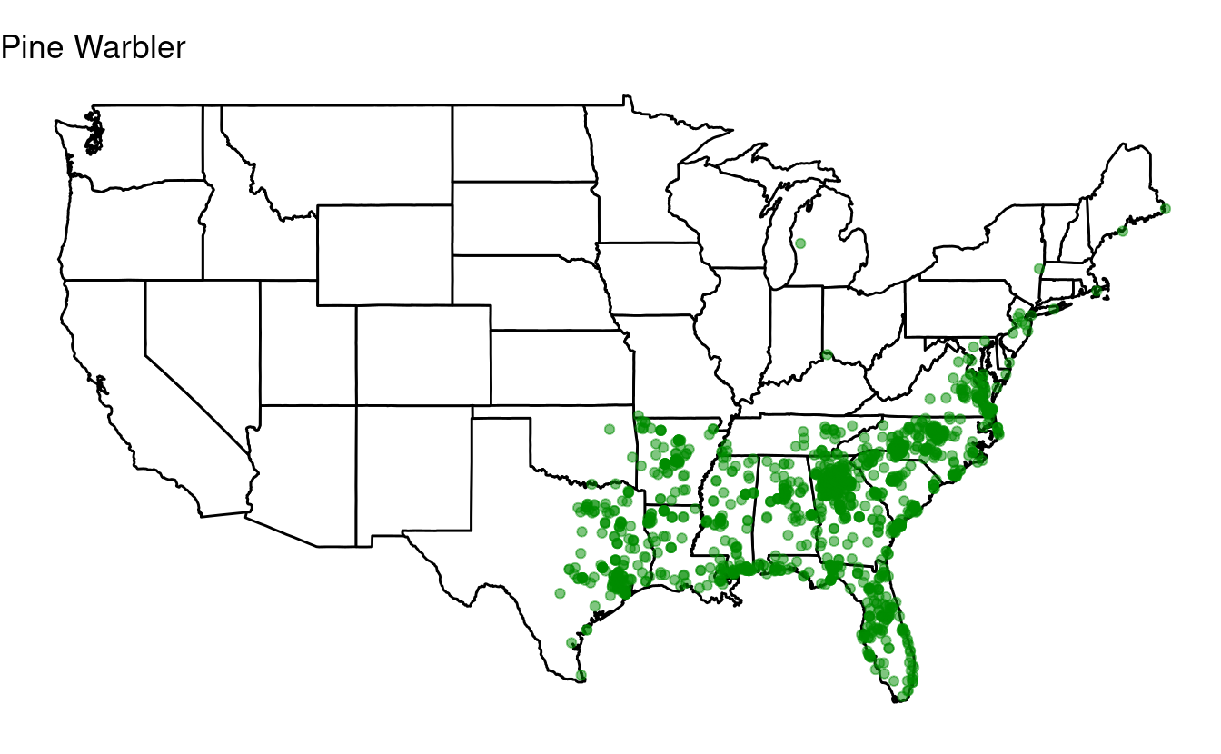
head(n = 10) # Take the top 10Next, loop over the top-10 species to produce a plot for each one of them.
Start with the code for the Carolina Chickadee, including the subsetting operation, and modify that.
Hints (click here)
-
In the subsetting operation where you select data for the focal species, replace “Carolina Chickadee” with whatever you name the variable (indicating an individual species) that you loop over.
Because this is a variable name, and not a string like “Carolina Chickadee”, don’t forget to omit the quotes.
-
You’ll also need to change the title with the looping variable.
Solution (click here)
for (one_species in top10) {

## Select just the data for one species:
one_bird_data <- birds[birds$species_en == one_species, ]
## Or in tidyverse-speak:
# one_bird_data <- birds %>% filter(species_en == one_species)

p <- ggplot(data = states,
            mapping = aes(x = long, y = lat, group = group)) +
  geom_polygon(color = "black", fill = "white") +
  geom_point(data = one_bird_data,
             aes(x = long, y = lat, group = NULL),
             color = "green4", alpha = 0.5) +
  coord_fixed(1.3) +
  labs(title = one_species) +  # Make sure to change this to the looping variable
  theme_void()
print(p)
}


Bonus exercise: if statements
if statements are similar in syntax to for loops, and are also considered a “control flow” structure. But their purpose is different from loops: instead of iterating, if statements do something once and they only do it when a condition is fulfilled.
For instance, we may want to check in a script whether a certain directory (folder) exists on our computer, and if it doesn’t, then we create the directory:
if (dir.exists('path/to/my/dir')) {
  warning("Oh my, the output directory doesn't exist yet!")
  dir.create('path/to/my/dir')
}
Inside the parentheses () after if should be a statement that evaluates to either TRUE or FALSE (dir.exists() will be TRUE if the directory exists, and FALSE if it does not). If it is TRUE, whatever is inside the curly braces {} will be executed, and if it is FALSE, what is inside the curly braces will be ignored.
if statements are commonly combined with for loops: we may want to only execute the functions in our loop for items in our collection that fulfill a certain condition:
for (one_number in 1:10) {
  if(one_number > 7) {
    print(one_number)
  }
}
#> [1] 8
#> [1] 9
#> [1] 10
In the example above, one number > 7 will only be TRUE for numbers larger than 7. This example is quite contrived, as it would have been easier (and faster!) to remove these items from the vector before the loop, but it hopefully gets the point across of how an if statement works.
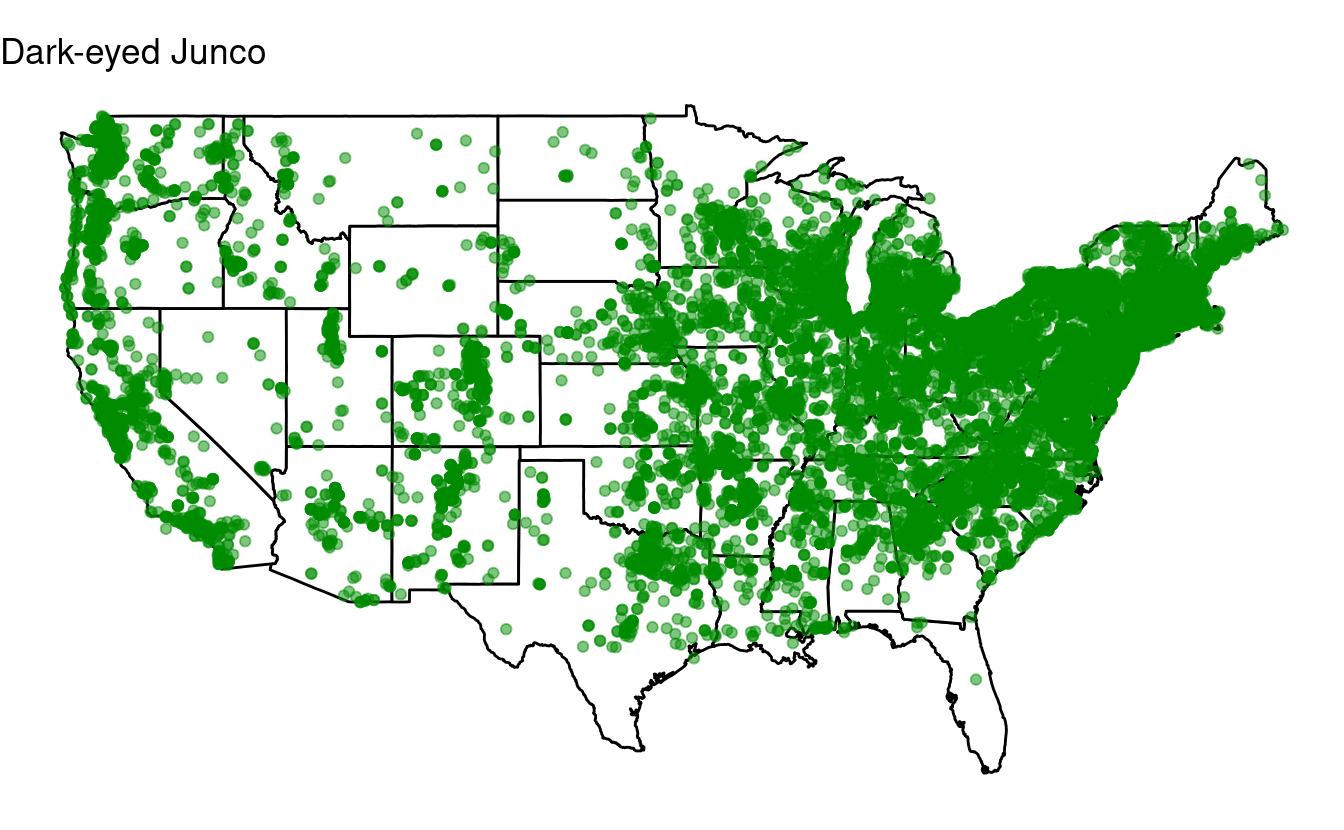
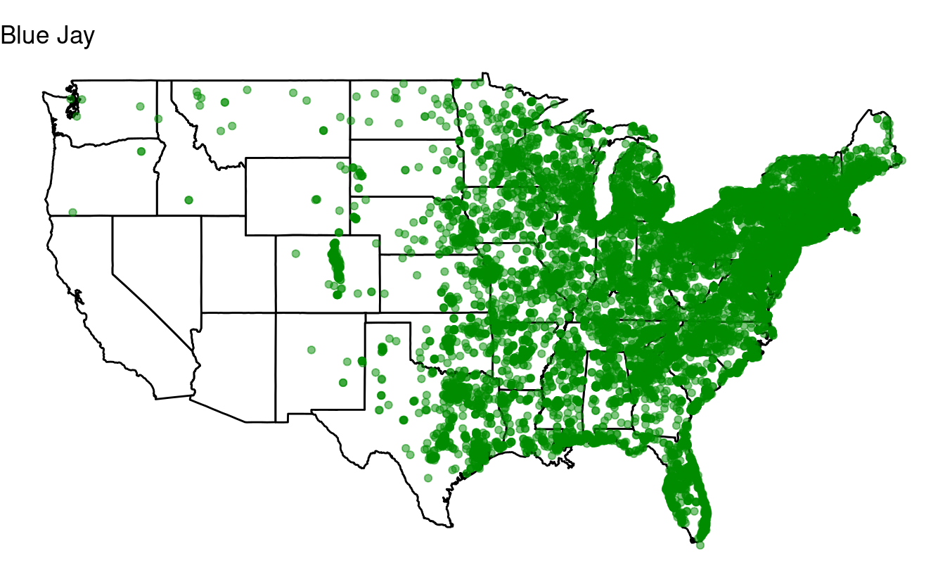
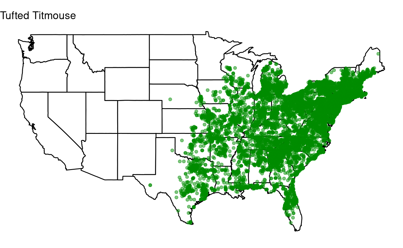
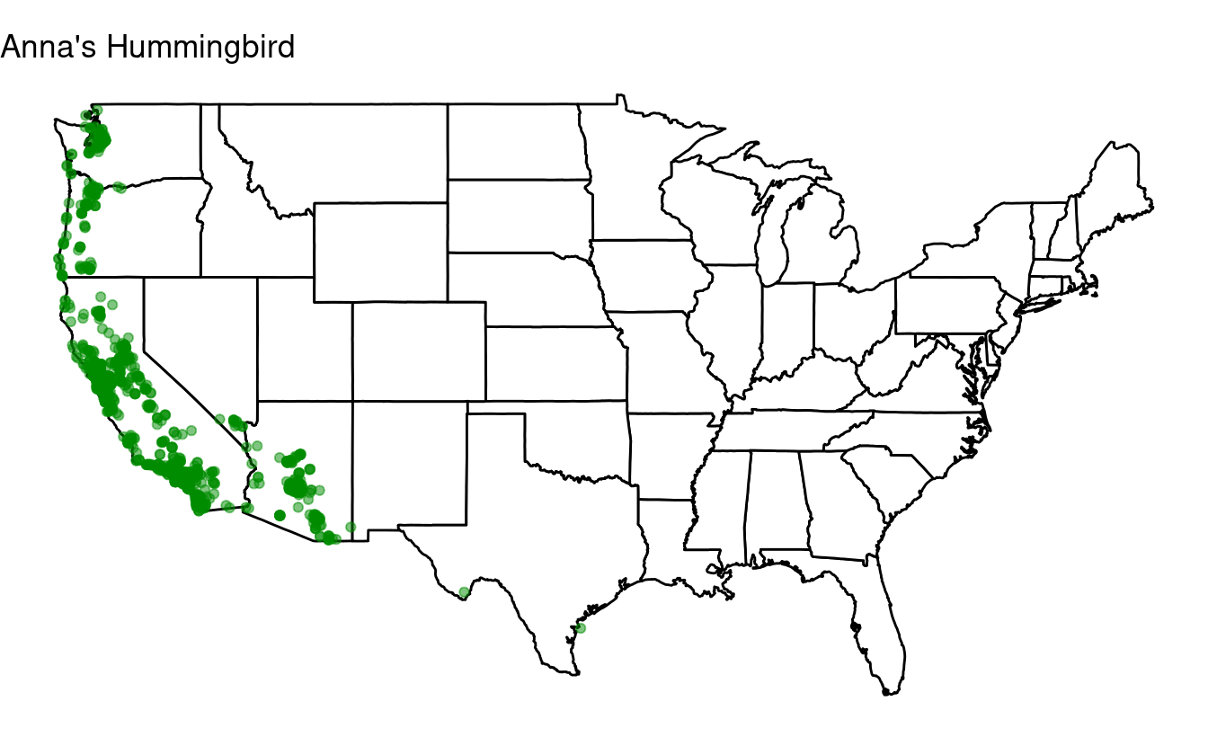
Many of the maps we produced in the previous exercise looked quite similar, with most species very widespread and a few restricted to the east of the US. Maybe if we select species that haven’t been seen in Ohio, we can find some other distributional patterns.
First, select the the top 50 most observed bird species, just like you did in exercise 2.
Then, use an if statement to create plots only for those top-50 birds that have not been seen in Ohio.
Solution (click here)
- Select the top-50 birds:
all_species <- birds %>%
  count(species_en, sort = TRUE) %>%
  pull(species_en) %>%
head(n = 50)- Loop over the species:
for (one_species in all_species) {

  ## Select the focal species:
  one_bird <- birds[birds$species_en == one_species, ]

  ## Create a data frame with only records from Ohio:
  one_bird_ohio <- one_bird[one_bird$stateProvince == 'Ohio', ]

  ## Test whether the data frame with only records from Ohio has any rows.
  ## If it does not, we create the map for the species in question:
  if(nrow(one_bird_ohio) == 0) {

    p <- ggplot(data = states,
           mapping = aes(x = long, y = lat, group = group)) +
      geom_polygon(color = "black", fill = "white") +
      geom_point(data = one_bird,
                 aes(x = long, y = lat, group = NULL),
                 color = "green4", alpha = 0.5) +
      coord_fixed(1.3) +
      labs(title = one_species) +
      theme_void()
    print(p)
    }
}

Going further
Base R data frame indexing
Extract a column as a vector:
## By name:
birds$lat
birds[['lat']]   # Equivalent, $ notation is shorthand

## By index (column number):
birds[[8]]
Extract one or more columns as a data frame using [row, column] notation,
with a leading comma ([, column]) meaning all rows:
## By name:
birds[, 'lat']   # dataframe['row_name', 'column_name']
birds[, c('lat', 'long')]

## By index (column numbers):
birds[, 8]       # dataframe[row_number, column_number]
birds[, c(8, 9)]
Subset rows by a condition, with a trailing comma ([row, ]) meaning all columns:
birds[birds$lat > 25, ]
birds[birds$species_en == 'Carolina Chickadee', ]
seq_along()
To loop over column indices, we have used 1:ncol() above, and to loop over vector indices, you could similarly use 1:length().
However, an alternative is seq_along(), which will create an index for you.
The advantage of seq_along() is thtat it will behave better when your vector accidentally has length 0 (because 1:length() will have 1 and 0 when the length is 0, and you’ll get odd-seeming errors).
Further reading
- Vectorization in R: Why? (Noam Ross, 2014)
- The Iteration chapter in Hadley Wickham’s R for Data Science (2017)