Session 2: dplyr core verbs
Using select, filter, mutate, arrange, and summarize
 Artwork by @allison_horst
Prep homework
Basic computer setup
-
If you didn’t already do this, please follow the Code Club Computer Setup instructions, which also has pointers for if you’re new to R or RStudio.
-
If you’re able to do so, please open RStudio a bit before Code Club starts – and in case you run into issues, please join the Zoom call early and we’ll troubleshoot.
New to dplyr?
If you’ve never used dplyr before (or even if you have), you may find this cheat sheet useful.
Getting Started
Want to download an R script with the content from today’s session?
# directory for Code Club Session 2:
dir.create("S02")

# directory for our script
# ("recursive" to create two levels at once.)
dir.create("S02/scripts/")

# save the url location for today's script
todays_R_script <- 'https://raw.githubusercontent.com/biodash/biodash.github.io/master/content/codeclub/02_dplyr-core-verbs/2_Dplyr_one-table_verbs.R'

# indicate the name of the new script file
Session2_dplyr_core <- "S02/scripts/Session2_script.R"

# go get that file!
download.file(url = todays_R_script,
              destfile = Session2_dplyr_core)
1 - What is data wrangling?
It has been estimated that the process of getting your data into the appropriate formats takes about 80% of the total time of analysis. We will talk about formatting as tidy data (e.g., such that each column is a single variable, each row is a single observation, and each cell is a single value, you can learn more about tidy data here) in a future session of Code Club.
The package dplyr, as part of the tidyverse has a number of very helpful functions that will help you get your data into a format suitable for your analysis.
What will we go over today
These five core dplyr() verbs will help you get wrangling.
select()- picks variables (i.e., columns) based on their namesfilter()- picks observations (i.e., rows) based on their valuesmutate()- makes new variables, keeps existing columnsarrange()- sorts rows based on values in columnssummarize()- reduces values down to a summary form
2 - Get ready to wrangle
Let’s get set up and grab some data so that we can get familiar with these verbs
- You can do this locally, or at OSC. You can find instructions if you are having trouble here.
First load your libraries.
library(tidyverse)

#> ── Attaching packages ─────────────────────────────────────── tidyverse 1.3.0 ──

#> ✔ ggplot2 3.3.2     ✔ purrr   0.3.4
#> ✔ tibble  3.0.4     ✔ dplyr   1.0.2
#> ✔ tidyr   1.1.2     ✔ stringr 1.4.0
#> ✔ readr   1.4.0     ✔ forcats 0.5.0

#> ── Conflicts ────────────────────────────────────────── tidyverse_conflicts() ──
#> ✖ dplyr::filter() masks stats::filter()
#> ✖ dplyr::lag()    masks stats::lag()
Then let’s access the iris dataset that comes pre-loaded in base R. We will take that data frame and assign it to a new object called iris_data. Then we will look at our data.
iris_data <- iris

# look at the first 6 rows, all columns
head(iris_data)

#>   Sepal.Length Sepal.Width Petal.Length Petal.Width Species
#> 1          5.1         3.5          1.4         0.2  setosa
#> 2          4.9         3.0          1.4         0.2  setosa
#> 3          4.7         3.2          1.3         0.2  setosa
#> 4          4.6         3.1          1.5         0.2  setosa
#> 5          5.0         3.6          1.4         0.2  setosa
#> 6          5.4         3.9          1.7         0.4  setosa


# check the structure of iris_data
glimpse(iris_data)

#> Rows: 150
#> Columns: 5
#> $ Sepal.Length <dbl> 5.1, 4.9, 4.7, 4.6, 5.0, 5.4, 4.6, 5.0, 4.4, 4.9, 5.4, 4…
#> $ Sepal.Width  <dbl> 3.5, 3.0, 3.2, 3.1, 3.6, 3.9, 3.4, 3.4, 2.9, 3.1, 3.7, 3…
#> $ Petal.Length <dbl> 1.4, 1.4, 1.3, 1.5, 1.4, 1.7, 1.4, 1.5, 1.4, 1.5, 1.5, 1…
#> $ Petal.Width  <dbl> 0.2, 0.2, 0.2, 0.2, 0.2, 0.4, 0.3, 0.2, 0.2, 0.1, 0.2, 0…
#> $ Species      <fct> setosa, setosa, setosa, setosa, setosa, setosa, setosa, …
This dataset contains the measurements (in cm) of Sepal.Length, Sepal.Width, Petal.Length, and Petal.Width for three different Species of iris, setosa, versicolor, and virginica.
3 - Using select()
select() allows you to pick certain columns to be included in your data frame.
We will create a dew data frame called iris_petals_species that includes the columns Species, Petal.Length and Petal.Width.
iris_petals_species <- iris_data %>%
  select(Species, Petal.Length, Petal.Width)
What does our new data frame look like?
head(iris_petals_species)

#>   Species Petal.Length Petal.Width
#> 1  setosa          1.4         0.2
#> 2  setosa          1.4         0.2
#> 3  setosa          1.3         0.2
#> 4  setosa          1.5         0.2
#> 5  setosa          1.4         0.2
#> 6  setosa          1.7         0.4
Note - look what happened to the order of the columns!
This is not the only way to select columns.
You could also subset by indexing with the square brackets, but you can see how much more readable using select() is. It’s nice not to have to refer back to remember what column is which index.
iris_data_indexing <- iris_data[,3:5]

head(iris_data_indexing)

#>   Petal.Length Petal.Width Species
#> 1          1.4         0.2  setosa
#> 2          1.4         0.2  setosa
#> 3          1.3         0.2  setosa
#> 4          1.5         0.2  setosa
#> 5          1.4         0.2  setosa
#> 6          1.7         0.4  setosa
4 - Using filter()
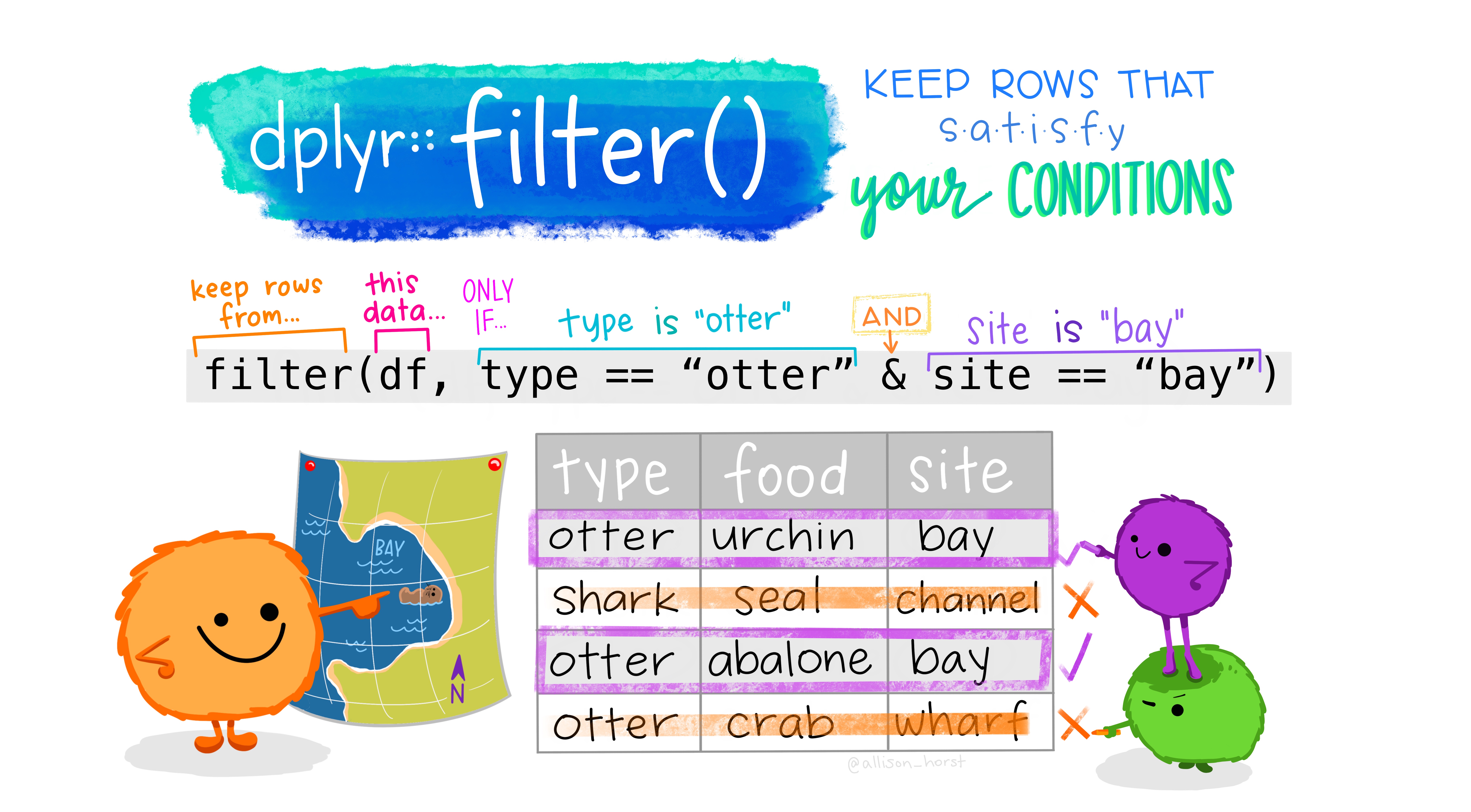
filter() allows you to pick certain observations (i.e, rows) based on their values to be included in your data frame.
We will create a new data frame that only includes information about the irises where their Species is setosa.
iris_setosa <- iris_data %>%
  filter(Species == "setosa")
Let’s check the dimensions of our data frame. Remember, our whole data set is 150 observations, and we are expecting 50 observations per Species.
dim(iris_setosa)

#> [1] 50  5
5 - Using mutate()
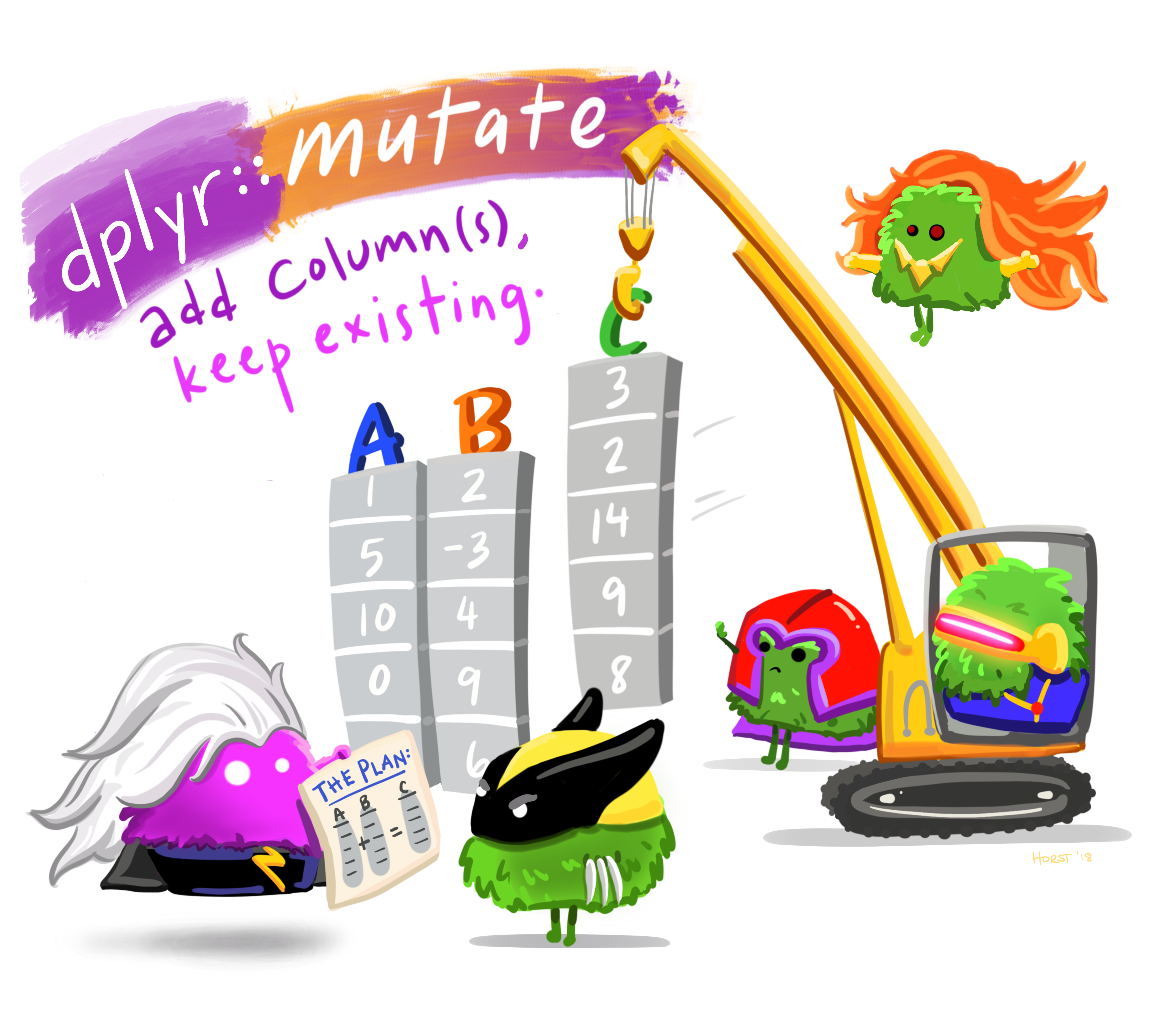
mutate() allows you to make new variables, while keeping all your existing columns.
Let’s make a new column that is the ratio of Sepal.Length/Sepal.Width
iris_sepal_length_to_width <- iris_data %>%
  mutate(Sepal.Length_div_Sepal.Width = Sepal.Length/Sepal.Width)
head(iris_sepal_length_to_width)

#>   Sepal.Length Sepal.Width Petal.Length Petal.Width Species
#> 1          5.1         3.5          1.4         0.2  setosa
#> 2          4.9         3.0          1.4         0.2  setosa
#> 3          4.7         3.2          1.3         0.2  setosa
#> 4          4.6         3.1          1.5         0.2  setosa
#> 5          5.0         3.6          1.4         0.2  setosa
#> 6          5.4         3.9          1.7         0.4  setosa
#>   Sepal.Length_div_Sepal.Width
#> 1                     1.457143
#> 2                     1.633333
#> 3                     1.468750
#> 4                     1.483871
#> 5                     1.388889
#> 6                     1.384615
Note – see the new column location
6 - Using arrange()
Very often you will want to order your data frame by some values. To do this, you can use arrange().
Let’s arrange the values in our iris_data by Sepal.Length.
iris_data_sort_Sepal.Length <- iris_data %>%
  arrange(Sepal.Length)

head(iris_data_sort_Sepal.Length)

#>   Sepal.Length Sepal.Width Petal.Length Petal.Width Species
#> 1          4.3         3.0          1.1         0.1  setosa
#> 2          4.4         2.9          1.4         0.2  setosa
#> 3          4.4         3.0          1.3         0.2  setosa
#> 4          4.4         3.2          1.3         0.2  setosa
#> 5          4.5         2.3          1.3         0.3  setosa
#> 6          4.6         3.1          1.5         0.2  setosa
What if we want to arrange by Sepal.Length, but within Species? We can do that using the helper group_by().
iris_data %>%
  group_by(Species) %>%
  arrange(Sepal.Length)

#> # A tibble: 150 x 5
#> # Groups:   Species [3]
#>    Sepal.Length Sepal.Width Petal.Length Petal.Width Species
#>           <dbl>       <dbl>        <dbl>       <dbl> <fct>
#>  1          4.3         3            1.1         0.1 setosa
#>  2          4.4         2.9          1.4         0.2 setosa
#>  3          4.4         3            1.3         0.2 setosa
#>  4          4.4         3.2          1.3         0.2 setosa
#>  5          4.5         2.3          1.3         0.3 setosa
#>  6          4.6         3.1          1.5         0.2 setosa
#>  7          4.6         3.4          1.4         0.3 setosa
#>  8          4.6         3.6          1           0.2 setosa
#>  9          4.6         3.2          1.4         0.2 setosa
#> 10          4.7         3.2          1.3         0.2 setosa
#> # … with 140 more rows
7 - Using summarize()
By using summarize(), you can create a new data frame that has the summary output you have requested.
We can calculate the mean Sepal.Length across our dataset.
iris_data %>%
  summarize(mean = mean(Sepal.Length))

#>       mean
#> 1 5.843333
What if we want to calculate means for each Species?
iris_data %>%
  group_by(Species) %>%
  summarize(mean = mean(Sepal.Length))

#> `summarise()` ungrouping output (override with `.groups` argument)

#> # A tibble: 3 x 2
#>   Species     mean
#>   <fct>      <dbl>
#> 1 setosa      5.01
#> 2 versicolor  5.94
#> 3 virginica   6.59
We can integrate some helper functions into our code to simply get out a variety of outputs. We can use across() to apply our summary aross a set of columns. I really like this function.
iris_data %>%
  group_by(Species) %>%
  summarize(across(where(is.numeric), mean))

#> `summarise()` ungrouping output (override with `.groups` argument)

#> # A tibble: 3 x 5
#>   Species    Sepal.Length Sepal.Width Petal.Length Petal.Width
#>   <fct>             <dbl>       <dbl>        <dbl>       <dbl>
#> 1 setosa             5.01        3.43         1.46       0.246
#> 2 versicolor         5.94        2.77         4.26       1.33
#> 3 virginica          6.59        2.97         5.55       2.03
This can also be useful for counting observations per group. Here, how many iris observations do we have per Species?
iris_data %>%
  group_by(Species) %>%
  tally()

#> # A tibble: 3 x 2
#>   Species        n
#>   <fct>      <int>
#> 1 setosa        50
#> 2 versicolor    50
#> 3 virginica     50


iris_data %>%
  count(Species)

#>      Species  n
#> 1     setosa 50
#> 2 versicolor 50
#> 3  virginica 50


iris_data %>%
  group_by(Species) %>%
  summarize(n = n())

#> `summarise()` ungrouping output (override with `.groups` argument)

#> # A tibble: 3 x 2
#>   Species        n
#>   <fct>      <int>
#> 1 setosa        50
#> 2 versicolor    50
#> 3 virginica     50
8 - Breakout rooms!
Read in data
Now you try! We are going to use the Great Backyard Birds dataset we downloaded two weeks ago and you will apply the functions we have learned above to investigate this dataset.
If you weren’t here for Session 1, get the birds data set.
# create a directory called S02
dir.create('S02')

# within S02, create a directory called data, within, a directory called birds
dir.create('data/birds/', recursive = TRUE)
Download the file from the internet.
# set the location of the file
birds_file_url <- 'https://raw.githubusercontent.com/biodash/biodash.github.io/master/assets/data/birds/backyard-birds_Ohio.tsv'

# set the path for the downloaded file
birds_file <- 'data/birds/backyard-birds_Ohio.tsv'

# download
download.file(url = birds_file_url, destfile = birds_file)
If you were here for Session 1, join back in! Let’s read in our data.
birds_file <- 'data/birds/backyard-birds_Ohio.tsv'
birds <- read_tsv(birds_file)

#>
#> ── Column specification ────────────────────────────────────────────────────────
#> cols(
#>   class = col_character(),
#>   order = col_character(),
#>   family = col_character(),
#>   genus = col_character(),
#>   species = col_character(),
#>   locality = col_character(),
#>   stateProvince = col_character(),
#>   decimalLatitude = col_double(),
#>   decimalLongitude = col_double(),
#>   eventDate = col_datetime(format = ""),
#>   species_en = col_character(),
#>   range = col_character()
#> )
Exercises
Below you can find our breakout room exercises for today.
Exercise 1
Investigate the structure of the birds dataset.
Solution (click here)
glimpse(birds)

#> Rows: 311,441
#> Columns: 12
#> $ class            <chr> "Aves", "Aves", "Aves", "Aves", "Aves", "Aves", "Ave…
#> $ order            <chr> "Passeriformes", "Passeriformes", "Passeriformes", "…
#> $ family           <chr> "Corvidae", "Corvidae", "Corvidae", "Corvidae", "Cor…
#> $ genus            <chr> "Cyanocitta", "Cyanocitta", "Cyanocitta", "Cyanocitt…
#> $ species          <chr> "Cyanocitta cristata", "Cyanocitta cristata", "Cyano…
#> $ locality         <chr> "44805 Ashland", "45244 Cincinnati", "44132 Euclid",…
#> $ stateProvince    <chr> "Ohio", "Ohio", "Ohio", "Ohio", "Ohio", "Ohio", "Ohi…
#> $ decimalLatitude  <dbl> 40.86166, 39.10666, 41.60768, 39.24236, 39.28207, 41…
#> $ decimalLongitude <dbl> -82.31558, -84.32972, -81.50085, -84.35545, -84.4688…
#> $ eventDate        <dttm> 2007-02-16, 2007-02-17, 2007-02-17, 2007-02-19, 200…
#> $ species_en       <chr> "Blue Jay", "Blue Jay", "Blue Jay", "Blue Jay", "Blu…
#> $ range            <chr> NA, NA, NA, NA, NA, NA, NA, NA, NA, NA, NA, NA, NA, …
Exercise 2
Create a new data frame that removes the column range.
Hints (click here)
Try using select(). Remember, you can tell select() what you want to keep, and what you want to remove.
Solutions (click here)
birds_no_range <- birds %>%
  select(-range)

head(birds_no_range)

#> # A tibble: 6 x 11
#>   class order family genus species locality stateProvince decimalLatitude
#>   <chr> <chr> <chr>  <chr> <chr>   <chr>    <chr>                   <dbl>
#> 1 Aves  Pass… Corvi… Cyan… Cyanoc… 44805 A… Ohio                     40.9
#> 2 Aves  Pass… Corvi… Cyan… Cyanoc… 45244 C… Ohio                     39.1
#> 3 Aves  Pass… Corvi… Cyan… Cyanoc… 44132 E… Ohio                     41.6
#> 4 Aves  Pass… Corvi… Cyan… Cyanoc… 45242 C… Ohio                     39.2
#> 5 Aves  Pass… Corvi… Cyan… Cyanoc… 45246 C… Ohio                     39.3
#> 6 Aves  Pass… Corvi… Cyan… Cyanoc… 44484 W… Ohio                     41.2
#> # … with 3 more variables: decimalLongitude <dbl>, eventDate <dttm>,
#> #   species_en <chr>
Exercise 3
How many unique species of birds have been observed?.
Hints (click here)
Try using summarize() with a group_by() helper.
Solutions (click here)
# using a combo of group_by() and summarize()
unique_birds <- birds %>%
  group_by(species_en) %>%
  summarize()

#> `summarise()` ungrouping output (override with `.groups` argument)


dim(unique_birds) # question - are there really 170 different birds observed?  take a look at this summary

#> [1] 170   1


# a one line, base R approach
length(unique(birds$species_en))

#> [1] 170


# another base R approach using distinct() and nrow()
birds %>%
  distinct(species_en) %>% # find distinct occurences
  nrow() # counts rows

#> [1] 170


# using n_distinct()
birds %>%
  summarize(n_distinct(species_en))

#> # A tibble: 1 x 1
#>   `n_distinct(species_en)`
#>                      <int>
#> 1                      170
Exercise 4
Exercise 5
How many times have any kind of eagle been observed?. Group hint: there are only Bald Eagle and Golden Eagle in this dataset.
Hints (click here)
There is a way to denote OR within filter().
More Hints (click here)
You denote OR by using the vertical bar.
Solutions (click here)
Exercise 6
What is the northern most location of the bird observations in Ohio?
Hints (click here)
Try using arrange(). You can arrange in both ascending and descending order. You can also use your Ohio knowledge to check if you’ve done this correctly.
Solutions (click here)
birds_sort_lat <- birds %>%
  arrange(-decimalLatitude)

head(birds_sort_lat)

#> # A tibble: 6 x 12
#>   class order family genus species locality stateProvince decimalLatitude
#>   <chr> <chr> <chr>  <chr> <chr>   <chr>    <chr>                   <dbl>
#> 1 Aves  Pass… Cardi… Card… Cardin… Conneaut Ohio                     41.9
#> 2 Aves  Pass… Ember… Zono… Zonotr… Conneaut Ohio                     41.9
#> 3 Aves  Colu… Colum… Zena… Zenaid… Conneaut Ohio                     41.9
#> 4 Aves  Pici… Picid… Dend… Dendro… Conneaut Ohio                     41.9
#> 5 Aves  Anse… Anati… Anas  Anas p… Conneaut Ohio                     41.9
#> 6 Aves  Pass… Turdi… Sial… Sialia… Conneaut Ohio                     41.9
#> # … with 4 more variables: decimalLongitude <dbl>, eventDate <dttm>,
#> #   species_en <chr>, range <chr>
Bonus time!
Bonus 1
What is the most commonly observed bird in Ohio?
Hints (click here)
Try using tally() and a little helper term.
Solutions (click here)
unique_birds_tally <- birds %>%
  group_by(species_en) %>%
  tally(sort = TRUE)

head(unique_birds_tally)

#> # A tibble: 6 x 2
#>   species_en            n
#>   <chr>             <int>
#> 1 Northern Cardinal 23064
#> 2 Mourning Dove     19135
#> 3 Dark-eyed Junco   18203
#> 4 Downy Woodpecker  17196
#> 5 House Sparrow     15939
#> 6 Blue Jay          15611


# another option
birds %>%
  count(species_en, sort = TRUE)

#> # A tibble: 170 x 2
#>    species_en                 n
#>    <chr>                  <int>
#>  1 Northern Cardinal      23064
#>  2 Mourning Dove          19135
#>  3 Dark-eyed Junco        18203
#>  4 Downy Woodpecker       17196
#>  5 House Sparrow          15939
#>  6 Blue Jay               15611
#>  7 American Goldfinch     14732
#>  8 House Finch            14551
#>  9 Tufted Titmouse        14409
#> 10 Black-capped Chickadee 13471
#> # … with 160 more rows
Bonus 2
What is the least commonly observed bird (or birds) in Ohio?
Hints (click here)
Try using the data frame you’ve created in the previous exercise.
Solutions (click here)
unique_birds_tally %>%
  arrange(n)

#> # A tibble: 170 x 2
#>    species_en               n
#>    <chr>                <int>
#>  1 Arctic Redpoll           1
#>  2 Clay-colored Sparrow     1
#>  3 Dickcissel               1
#>  4 Eurasian Wigeon          1
#>  5 Great Egret              1
#>  6 Green Heron              1
#>  7 Grey Partridge           1
#>  8 Harris's Sparrow         1
#>  9 Lesser Yellowlegs        1
#> 10 Lincoln's Sparrow        1
#> # … with 160 more rows


# or, if you knew the rarest was those observed only once
unique_birds_tally %>%
  filter(n == 1)

#> # A tibble: 19 x 2
#>    species_en                        n
#>    <chr>                         <int>
#>  1 Arctic Redpoll                    1
#>  2 Clay-colored Sparrow              1
#>  3 Dickcissel                        1
#>  4 Eurasian Wigeon                   1
#>  5 Great Egret                       1
#>  6 Green Heron                       1
#>  7 Grey Partridge                    1
#>  8 Harris's Sparrow                  1
#>  9 Lesser Yellowlegs                 1
#> 10 Lincoln's Sparrow                 1
#> 11 Loggerhead Shrike                 1
#> 12 Nelson's Sparrow                  1
#> 13 Northern Rough-winged Swallow     1
#> 14 Orchard Oriole                    1
#> 15 Prairie Falcon                    1
#> 16 Red-throated Loon                 1
#> 17 Ross's Goose                      1
#> 18 Warbling Vireo                    1
#> 19 Western Osprey                    1
Bonus 3
In what year were the most Bald Eagles observed?
Hints (click here)
You may want to convert your date column to a more simplified year-only date. Check out the package lubridate.Solutions (click here)
library(lubridate)

#>
#> Attaching package: 'lubridate'

#> The following objects are masked from 'package:base':
#>
#>     date, intersect, setdiff, union

birds_bald_eagle_year <- birds_bald_eagle %>%
  mutate(year = year(eventDate)) %>% # year() takes a date and outputs only year
  group_by(year) %>%
  tally()

arrange(birds_bald_eagle_year, -n)

#> # A tibble: 11 x 2
#>     year     n
#>    <dbl> <int>
#>  1  2008    81
#>  2  2006    66
#>  3  2009    58
#>  4  2007    40
#>  5  2005    30
#>  6  2004    26
#>  7  2000    23
#>  8  2001    23
#>  9  2003    15
#> 10  2002    14
#> 11  1999     5