Session 3: Joining Datasets
Using join functions to merge pairs of datasets
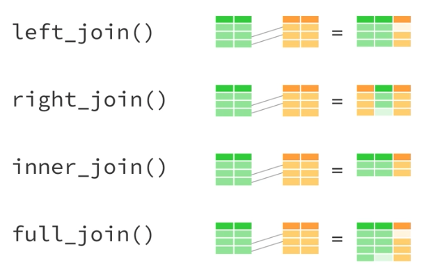 Image from https://rpubs.com/williamsurles/293454
New To Code Club?
-
First, check out the Code Club Computer Setup instructions, which also has some pointers that might be helpful if you’re new to R or RStudio.
-
Please open RStudio before Code Club to test things out – if you run into issues, join the Zoom call early and we’ll troubleshoot.
Session Goals
- Differentiate between different types of joins…
inner_join()full_join()left_join()right_join()
- Use a join function to add new variables to the birds dataset
- Keep practicing with dplyr core verbs from last week, esp…
select()filter()
- Answer the question “What Ohio bird species have the longest and shortest average lifespans?”.
Intro: Merging/Joining Datasets
Sometimes you don’t have all your data in the same place. For example, maybe you have multiple Excel sheets for a project - each storing a different type of data for the same set of samples. Or maybe you’re interested in analyzing various metrics for US states and are getting the data from different places online - economic data from one database, climate data from another, and so on. As part of the process of data wrangling, it’s often useful to merge the separate datasets together according to a variable they share, possibly “SampleID” or “State Name” for the two above examples, respectively. R offers several ways to do this, but we’ll focus here on the set of *_join() functions available in dplyr. They include…
inner_join()full_join()left_join()right_join()semi_join()anti_join()
Check out the ‘Combine Data Sets’ section of this cheat sheet for a brief look at these functions.
You can also get more details here, or, as with any R function, by accessing the function’s documentation inside R with the ‘?’. For example, type ?inner_join at your R prompt and hit Enter. (Make sure the package the function comes from is loaded first! In this case, you need dplyr, which is loaded as part of tidyverse.)
Examples
Below we’ll go through a few examples of joins. You’re welcome to follow along and run this code on your own, but it’s not necessary - the exercises in the breakout rooms are independent of these examples and will give you a chance to try these things out on your own.
If you want to follow along, you can find the code here.
Since the *_join() functions come from the dplyr package, which is part of tidyverse, I’ll load that first…
The National Health and Nutrition Examination Survey (NHANES) dataset contains survey data obtained annually from ~5,000 individuals on a variety of health and lifestyle-related metrics. A subset of the data are available as an R package - install and load it…
install.packages("NHANES", repos = "http://cran.us.r-project.org")

#>
#> The downloaded binary packages are in
#>   /var/folders/s7/y_mgh3c54h9fjcyw9wqdkb8x4zs_jy/T//RtmpdHHxzY/downloaded_packages

library(NHANES)
Now preview the dataset…
glimpse(NHANES)

#> Rows: 10,000
#> Columns: 76
#> $ ID               <int> 51624, 51624, 51624, 51625, 51630, 51638, 51646, 516…
#> $ SurveyYr         <fct> 2009_10, 2009_10, 2009_10, 2009_10, 2009_10, 2009_10…
#> $ Gender           <fct> male, male, male, male, female, male, male, female, …
#> $ Age              <int> 34, 34, 34, 4, 49, 9, 8, 45, 45, 45, 66, 58, 54, 10,…
#> $ AgeDecade        <fct>  30-39,  30-39,  30-39,  0-9,  40-49,  0-9,  0-9,  4…
#> $ AgeMonths        <int> 409, 409, 409, 49, 596, 115, 101, 541, 541, 541, 795…
#> $ Race1            <fct> White, White, White, Other, White, White, White, Whi…
#> $ Race3            <fct> NA, NA, NA, NA, NA, NA, NA, NA, NA, NA, NA, NA, NA, …
#> $ Education        <fct> High School, High School, High School, NA, Some Coll…
#> $ MaritalStatus    <fct> Married, Married, Married, NA, LivePartner, NA, NA, …
#> $ HHIncome         <fct> 25000-34999, 25000-34999, 25000-34999, 20000-24999, …
#> $ HHIncomeMid      <int> 30000, 30000, 30000, 22500, 40000, 87500, 60000, 875…
#> $ Poverty          <dbl> 1.36, 1.36, 1.36, 1.07, 1.91, 1.84, 2.33, 5.00, 5.00…
#> $ HomeRooms        <int> 6, 6, 6, 9, 5, 6, 7, 6, 6, 6, 5, 10, 6, 10, 10, 4, 3…
#> $ HomeOwn          <fct> Own, Own, Own, Own, Rent, Rent, Own, Own, Own, Own, …
#> $ Work             <fct> NotWorking, NotWorking, NotWorking, NA, NotWorking, …
#> $ Weight           <dbl> 87.4, 87.4, 87.4, 17.0, 86.7, 29.8, 35.2, 75.7, 75.7…
#> $ Length           <dbl> NA, NA, NA, NA, NA, NA, NA, NA, NA, NA, NA, NA, NA, …
#> $ HeadCirc         <dbl> NA, NA, NA, NA, NA, NA, NA, NA, NA, NA, NA, NA, NA, …
#> $ Height           <dbl> 164.7, 164.7, 164.7, 105.4, 168.4, 133.1, 130.6, 166…
#> $ BMI              <dbl> 32.22, 32.22, 32.22, 15.30, 30.57, 16.82, 20.64, 27.…
#> $ BMICatUnder20yrs <fct> NA, NA, NA, NA, NA, NA, NA, NA, NA, NA, NA, NA, NA, …
#> $ BMI_WHO          <fct> 30.0_plus, 30.0_plus, 30.0_plus, 12.0_18.5, 30.0_plu…
#> $ Pulse            <int> 70, 70, 70, NA, 86, 82, 72, 62, 62, 62, 60, 62, 76, …
#> $ BPSysAve         <int> 113, 113, 113, NA, 112, 86, 107, 118, 118, 118, 111,…
#> $ BPDiaAve         <int> 85, 85, 85, NA, 75, 47, 37, 64, 64, 64, 63, 74, 85, …
#> $ BPSys1           <int> 114, 114, 114, NA, 118, 84, 114, 106, 106, 106, 124,…
#> $ BPDia1           <int> 88, 88, 88, NA, 82, 50, 46, 62, 62, 62, 64, 76, 86, …
#> $ BPSys2           <int> 114, 114, 114, NA, 108, 84, 108, 118, 118, 118, 108,…
#> $ BPDia2           <int> 88, 88, 88, NA, 74, 50, 36, 68, 68, 68, 62, 72, 88, …
#> $ BPSys3           <int> 112, 112, 112, NA, 116, 88, 106, 118, 118, 118, 114,…
#> $ BPDia3           <int> 82, 82, 82, NA, 76, 44, 38, 60, 60, 60, 64, 76, 82, …
#> $ Testosterone     <dbl> NA, NA, NA, NA, NA, NA, NA, NA, NA, NA, NA, NA, NA, …
#> $ DirectChol       <dbl> 1.29, 1.29, 1.29, NA, 1.16, 1.34, 1.55, 2.12, 2.12, …
#> $ TotChol          <dbl> 3.49, 3.49, 3.49, NA, 6.70, 4.86, 4.09, 5.82, 5.82, …
#> $ UrineVol1        <int> 352, 352, 352, NA, 77, 123, 238, 106, 106, 106, 113,…
#> $ UrineFlow1       <dbl> NA, NA, NA, NA, 0.094, 1.538, 1.322, 1.116, 1.116, 1…
#> $ UrineVol2        <int> NA, NA, NA, NA, NA, NA, NA, NA, NA, NA, NA, NA, NA, …
#> $ UrineFlow2       <dbl> NA, NA, NA, NA, NA, NA, NA, NA, NA, NA, NA, NA, NA, …
#> $ Diabetes         <fct> No, No, No, No, No, No, No, No, No, No, No, No, No, …
#> $ DiabetesAge      <int> NA, NA, NA, NA, NA, NA, NA, NA, NA, NA, NA, NA, NA, …
#> $ HealthGen        <fct> Good, Good, Good, NA, Good, NA, NA, Vgood, Vgood, Vg…
#> $ DaysPhysHlthBad  <int> 0, 0, 0, NA, 0, NA, NA, 0, 0, 0, 10, 0, 4, NA, NA, 0…
#> $ DaysMentHlthBad  <int> 15, 15, 15, NA, 10, NA, NA, 3, 3, 3, 0, 0, 0, NA, NA…
#> $ LittleInterest   <fct> Most, Most, Most, NA, Several, NA, NA, None, None, N…
#> $ Depressed        <fct> Several, Several, Several, NA, Several, NA, NA, None…
#> $ nPregnancies     <int> NA, NA, NA, NA, 2, NA, NA, 1, 1, 1, NA, NA, NA, NA, …
#> $ nBabies          <int> NA, NA, NA, NA, 2, NA, NA, NA, NA, NA, NA, NA, NA, N…
#> $ Age1stBaby       <int> NA, NA, NA, NA, 27, NA, NA, NA, NA, NA, NA, NA, NA, …
#> $ SleepHrsNight    <int> 4, 4, 4, NA, 8, NA, NA, 8, 8, 8, 7, 5, 4, NA, 5, 7, …
#> $ SleepTrouble     <fct> Yes, Yes, Yes, NA, Yes, NA, NA, No, No, No, No, No, …
#> $ PhysActive       <fct> No, No, No, NA, No, NA, NA, Yes, Yes, Yes, Yes, Yes,…
#> $ PhysActiveDays   <int> NA, NA, NA, NA, NA, NA, NA, 5, 5, 5, 7, 5, 1, NA, 2,…
#> $ TVHrsDay         <fct> NA, NA, NA, NA, NA, NA, NA, NA, NA, NA, NA, NA, NA, …
#> $ CompHrsDay       <fct> NA, NA, NA, NA, NA, NA, NA, NA, NA, NA, NA, NA, NA, …
#> $ TVHrsDayChild    <int> NA, NA, NA, 4, NA, 5, 1, NA, NA, NA, NA, NA, NA, 4, …
#> $ CompHrsDayChild  <int> NA, NA, NA, 1, NA, 0, 6, NA, NA, NA, NA, NA, NA, 3, …
#> $ Alcohol12PlusYr  <fct> Yes, Yes, Yes, NA, Yes, NA, NA, Yes, Yes, Yes, Yes, …
#> $ AlcoholDay       <int> NA, NA, NA, NA, 2, NA, NA, 3, 3, 3, 1, 2, 6, NA, NA,…
#> $ AlcoholYear      <int> 0, 0, 0, NA, 20, NA, NA, 52, 52, 52, 100, 104, 364, …
#> $ SmokeNow         <fct> No, No, No, NA, Yes, NA, NA, NA, NA, NA, No, NA, NA,…
#> $ Smoke100         <fct> Yes, Yes, Yes, NA, Yes, NA, NA, No, No, No, Yes, No,…
#> $ Smoke100n        <fct> Smoker, Smoker, Smoker, NA, Smoker, NA, NA, Non-Smok…
#> $ SmokeAge         <int> 18, 18, 18, NA, 38, NA, NA, NA, NA, NA, 13, NA, NA, …
#> $ Marijuana        <fct> Yes, Yes, Yes, NA, Yes, NA, NA, Yes, Yes, Yes, NA, Y…
#> $ AgeFirstMarij    <int> 17, 17, 17, NA, 18, NA, NA, 13, 13, 13, NA, 19, 15, …
#> $ RegularMarij     <fct> No, No, No, NA, No, NA, NA, No, No, No, NA, Yes, Yes…
#> $ AgeRegMarij      <int> NA, NA, NA, NA, NA, NA, NA, NA, NA, NA, NA, 20, 15, …
#> $ HardDrugs        <fct> Yes, Yes, Yes, NA, Yes, NA, NA, No, No, No, No, Yes,…
#> $ SexEver          <fct> Yes, Yes, Yes, NA, Yes, NA, NA, Yes, Yes, Yes, Yes, …
#> $ SexAge           <int> 16, 16, 16, NA, 12, NA, NA, 13, 13, 13, 17, 22, 12, …
#> $ SexNumPartnLife  <int> 8, 8, 8, NA, 10, NA, NA, 20, 20, 20, 15, 7, 100, NA,…
#> $ SexNumPartYear   <int> 1, 1, 1, NA, 1, NA, NA, 0, 0, 0, NA, 1, 1, NA, NA, 1…
#> $ SameSex          <fct> No, No, No, NA, Yes, NA, NA, Yes, Yes, Yes, No, No, …
#> $ SexOrientation   <fct> Heterosexual, Heterosexual, Heterosexual, NA, Hetero…
#> $ PregnantNow      <fct> NA, NA, NA, NA, NA, NA, NA, NA, NA, NA, NA, NA, NA, …
To try out merging/joining, we’ll create two separate data frames by pulling out some variables from this NHANES dataset. One will contain demographic variables, and the other with have some physical measurements. Then we’ll join them back together. Let’s create the two sub-datasets first…
#Filter out rows with data from 2009-2010 and Age > 5,
#select a subset (4) of the variables, then get rid of
#all duplicate rows. Assign the output to object 'dem_data'.
dem_data <- NHANES %>%
            filter(SurveyYr == "2009_10") %>%
            filter(Age > 5) %>%
            select(ID, Gender, Age, Education) %>%
            distinct()

#similar as above, but with a different filter and
#selecting different variables. Save as 'phys_data'
phys_data <- NHANES %>%
             filter(SurveyYr == "2009_10") %>%
             filter(Height < 180)  %>%
             select(ID, Height, BMI, Pulse) %>%
             distinct()
Now explore them a bit…
#view the first 6 rows of each - note the shared ID column
head(dem_data)

#> # A tibble: 6 x 4
#>      ID Gender   Age Education
#>   <int> <fct>  <int> <fct>
#> 1 51624 male      34 High School
#> 2 51630 female    49 Some College
#> 3 51638 male       9 NA
#> 4 51646 male       8 NA
#> 5 51647 female    45 College Grad
#> 6 51654 male      66 Some College

head(phys_data)

#> # A tibble: 6 x 4
#>      ID Height   BMI Pulse
#>   <int>  <dbl> <dbl> <int>
#> 1 51624   165.  32.2    70
#> 2 51625   105.  15.3    NA
#> 3 51630   168.  30.6    86
#> 4 51638   133.  16.8    82
#> 5 51646   131.  20.6    72
#> 6 51647   167.  27.2    62

#preview in another way - note the different numbers of observations (rows)
glimpse(dem_data)

#> Rows: 3,217
#> Columns: 4
#> $ ID        <int> 51624, 51630, 51638, 51646, 51647, 51654, 51656, 51657, 516…
#> $ Gender    <fct> male, female, male, male, female, male, male, male, female,…
#> $ Age       <int> 34, 49, 9, 8, 45, 66, 58, 54, 10, 58, 50, 9, 33, 60, 16, 56…
#> $ Education <fct> High School, Some College, NA, NA, College Grad, Some Colle…

glimpse(phys_data)

#> Rows: 3,021
#> Columns: 4
#> $ ID     <int> 51624, 51625, 51630, 51638, 51646, 51647, 51654, 51657, 51659,…
#> $ Height <dbl> 164.7, 105.4, 168.4, 133.1, 130.6, 166.7, 169.5, 169.4, 141.8,…
#> $ BMI    <dbl> 32.22, 15.30, 30.57, 16.82, 20.64, 27.24, 23.67, 26.03, 19.20,…
#> $ Pulse  <int> 70, NA, 86, 82, 72, 62, 60, 76, 80, 94, 74, 92, 84, 76, 64, 70…
Let’s use the shared ID column to join the two datasets together. We’ll do this in 4 different ways to compare different types of joins: inner_join(), left_join(), right_join(), and full_join(). Pay attention to the number of rows in the joined dataset each time and how it relates to the number of rows in each of the two individual datasets.
The basic structure of the dplyr *_join() functions is…
*_join(dataframe 'x', dataframe 'y', by = shared column name)
1 - inner_join()
#perform an inner join
join_inner <- inner_join(dem_data, phys_data, by = "ID")

#preview the new object
head(join_inner)

#> # A tibble: 6 x 7
#>      ID Gender   Age Education    Height   BMI Pulse
#>   <int> <fct>  <int> <fct>         <dbl> <dbl> <int>
#> 1 51624 male      34 High School    165.  32.2    70
#> 2 51630 female    49 Some College   168.  30.6    86
#> 3 51638 male       9 NA             133.  16.8    82
#> 4 51646 male       8 NA             131.  20.6    72
#> 5 51647 female    45 College Grad   167.  27.2    62
#> 6 51654 male      66 Some College   170.  23.7    60

#get dimensions
dim(join_inner)

#> [1] 2806    7
2 - left_join()
#perform an left join
join_left <- left_join(dem_data, phys_data, by = "ID")

#preview the new object
head(join_left)

#> # A tibble: 6 x 7
#>      ID Gender   Age Education    Height   BMI Pulse
#>   <int> <fct>  <int> <fct>         <dbl> <dbl> <int>
#> 1 51624 male      34 High School    165.  32.2    70
#> 2 51630 female    49 Some College   168.  30.6    86
#> 3 51638 male       9 NA             133.  16.8    82
#> 4 51646 male       8 NA             131.  20.6    72
#> 5 51647 female    45 College Grad   167.  27.2    62
#> 6 51654 male      66 Some College   170.  23.7    60

#get dimensions
dim(join_left)

#> [1] 3217    7
3 - right_join()
#perform an right join
join_right <- right_join(dem_data, phys_data, by = "ID")

#preview the new object
head(join_right)

#> # A tibble: 6 x 7
#>      ID Gender   Age Education    Height   BMI Pulse
#>   <int> <fct>  <int> <fct>         <dbl> <dbl> <int>
#> 1 51624 male      34 High School    165.  32.2    70
#> 2 51630 female    49 Some College   168.  30.6    86
#> 3 51638 male       9 NA             133.  16.8    82
#> 4 51646 male       8 NA             131.  20.6    72
#> 5 51647 female    45 College Grad   167.  27.2    62
#> 6 51654 male      66 Some College   170.  23.7    60

#get dimensions
dim(join_right)

#> [1] 3021    7
4 - full_join()
#perform an full join
join_full <- full_join(dem_data, phys_data, by = "ID")

#preview the new object
head(join_full)

#> # A tibble: 6 x 7
#>      ID Gender   Age Education    Height   BMI Pulse
#>   <int> <fct>  <int> <fct>         <dbl> <dbl> <int>
#> 1 51624 male      34 High School    165.  32.2    70
#> 2 51630 female    49 Some College   168.  30.6    86
#> 3 51638 male       9 NA             133.  16.8    82
#> 4 51646 male       8 NA             131.  20.6    72
#> 5 51647 female    45 College Grad   167.  27.2    62
#> 6 51654 male      66 Some College   170.  23.7    60

#get dimensions
dim(join_full)

#> [1] 3432    7
Breakout rooms
We’re going to add to our backyard birds dataset. I found a dataset that has life history data for a large number of species (birds and others). We’ll use species names to merge some of these life history variables in to the occurrence data we already have.
If you’re new and haven’t yet gotten the backyard bird dataset, get it first by running the code below. Otherwise, you can skip this step…
# create a directory called data that contains a subdirectory called birds
dir.create('data/birds/', recursive = TRUE)

# set the location of the file
birds_file_url <-
'https://raw.githubusercontent.com/biodash/biodash.github.io/master/assets/data/birds/backyard-birds_Ohio.tsv'

# set the path for the downloaded file
birds_file <- 'data/birds/backyard-birds_Ohio.tsv'
#download
download.file(url = birds_file_url, destfile = birds_file)
Now (everybody), read in the bird data for this session…
birds_file <- 'data/birds/backyard-birds_Ohio.tsv'
birds <- read_tsv(birds_file)

#> Parsed with column specification:
#> cols(
#>   class = col_character(),
#>   order = col_character(),
#>   family = col_character(),
#>   genus = col_character(),
#>   species = col_character(),
#>   locality = col_character(),
#>   stateProvince = col_character(),
#>   decimalLatitude = col_double(),
#>   decimalLongitude = col_double(),
#>   eventDate = col_datetime(format = ""),
#>   species_en = col_character(),
#>   range = col_character()
#> )
Exercise 1
Reduce the backyard bird dataset and keep just the following columns: species, locality, stateProvince, eventDate, species_en
Hints (click here)
Use select() to pull out the columns you want.
Solution (click here)
birds <- birds %>% select(species, locality, stateProvince, eventDate, species_en)
Exercise 2
Check to make sure things look right - how many columns does the birds dataset now have?
Hints (click here)
Use the dim() function. Or the ncol() function. Or glimpse(). Or head(). Or str(). Or even summary(). There’s lots of ways to do this.
Exercise 3
Now download and read in the new life history dataset (tab separated) available at https://github.com/biodash/biodash.github.io/raw/master/assets/data/birds/esa_life_history_data_cc.tsv. Then explore it a bit - how many rows and columns are there?
Hints (click here)
Use the download.file() function like we did previously for the bird dataset. You’ll need to define the arguments ‘url’ and ‘destfile’ inside the parentheses. You can put the file anywhere you want, but I’d suggest in the same directory as the bird file we got, so, for example, the destination file could be “data/birds/life_history_data.tsv”.
Solution (click here)
#download the file from online and save it as a '.tsv' file (since it's tab delimited)
download.file(url = "https://github.com/biodash/biodash.github.io/raw/master/assets/data/birds/esa_life_history_data_cc.tsv",
destfile = "data/birds/life_history_data.tsv")

#read the data in to R as an object named 'life_hist'
life_hist <- read_tsv(file = "data/birds/life_history_data.tsv")

#> Parsed with column specification:
#> cols(
#>   class = col_character(),
#>   order = col_character(),
#>   family = col_character(),
#>   genus = col_character(),
#>   species = col_character(),
#>   common_name = col_character(),
#>   female_maturity_d = col_double(),
#>   litter_or_clutch_size_n = col_double(),
#>   litters_or_clutches_per_y = col_double(),
#>   adult_body_mass_g = col_double(),
#>   maximum_longevity_y = col_double(),
#>   egg_mass_g = col_double(),
#>   incubation_d = col_double(),
#>   fledging_age_d = col_double(),
#>   longevity_y = col_double(),
#>   adult_svl_cm = col_double()
#> )


#preview the data
glimpse(life_hist)

#> Rows: 21,322
#> Columns: 16
#> $ class                     <chr> "Aves", "Aves", "Aves", "Aves", "Aves", "Av…
#> $ order                     <chr> "Accipitriformes", "Accipitriformes", "Acci…
#> $ family                    <chr> "Accipitridae", "Accipitridae", "Accipitrid…
#> $ genus                     <chr> "Accipiter", "Accipiter", "Accipiter", "Acc…
#> $ species                   <chr> "Accipiter albogularis", "Accipiter badius"…
#> $ common_name               <chr> "Pied Goshawk", "Shikra", "Bicolored Hawk",…
#> $ female_maturity_d         <dbl> NA, 363.468, NA, NA, 363.468, NA, NA, 547.8…
#> $ litter_or_clutch_size_n   <dbl> NA, 3.250, 2.700, NA, 4.000, NA, 2.700, 4.2…
#> $ litters_or_clutches_per_y <dbl> NA, 1, NA, NA, 1, NA, NA, 1, NA, 1, NA, 1, …
#> $ adult_body_mass_g         <dbl> 251.500, 140.000, 345.000, 142.000, 203.500…
#> $ maximum_longevity_y       <dbl> NA, NA, NA, NA, NA, NA, NA, 19.90000, NA, 2…
#> $ egg_mass_g                <dbl> NA, 21.00, 32.00, NA, 21.85, NA, 32.00, 19.…
#> $ incubation_d              <dbl> NA, 30.00, NA, NA, 32.50, NA, NA, 33.00, NA…
#> $ fledging_age_d            <dbl> NA, 32.00, NA, NA, 42.50, NA, NA, 24.25, NA…
#> $ longevity_y               <dbl> NA, NA, NA, NA, NA, NA, NA, 12.58333, NA, 1…
#> $ adult_svl_cm              <dbl> NA, 30.00, 39.50, NA, 33.50, NA, 39.50, 29.…
Exercise 4
This new dataset contains life history data for more than just birds. What Classes of organisms are represented in the ‘Class’ variable?
Hints (click here)
Try using a combination of the select() and distinct() functions to pull out the column you’re interested in, and then to get the distinct values, respectively.
Solutions (click here)
life_hist %>% select(class) %>% distinct()

#> # A tibble: 3 x 1
#>   class
#>   <chr>
#> 1 Aves
#> 2 Mammalia
#> 3 Reptilia
Exercise 5
Reduce the life history dataset down to keep just the rows for Class Aves and the columns species, adult_body_mass_g, adult_svl_cm, longevity_y, litter_or_clutch_size_n. What are the dimensions now?
Hints (click here)
Use filter() along with an appropriate logical expression to keep the rows we want. Use select() to get the desired columns.
Solutions (click here)
Exercise 6
Preview each dataset again, just to make sure you’re clear about what’s in each one. Are there any columns that are shared between the two?
Hints (click here)
Consider glimpse() or head() to preview the datasets (tibbles/data frames). If you want to use a function to find shared columns, try a combination of intersect() and names().
Solutions (click here)
glimpse(birds)

#> Rows: 311,441
#> Columns: 12
#> $ class            <chr> "Aves", "Aves", "Aves", "Aves", "Aves", "Aves", "Ave…
#> $ order            <chr> "Passeriformes", "Passeriformes", "Passeriformes", "…
#> $ family           <chr> "Corvidae", "Corvidae", "Corvidae", "Corvidae", "Cor…
#> $ genus            <chr> "Cyanocitta", "Cyanocitta", "Cyanocitta", "Cyanocitt…
#> $ species          <chr> "Cyanocitta cristata", "Cyanocitta cristata", "Cyano…
#> $ locality         <chr> "44805 Ashland", "45244 Cincinnati", "44132 Euclid",…
#> $ stateProvince    <chr> "Ohio", "Ohio", "Ohio", "Ohio", "Ohio", "Ohio", "Ohi…
#> $ decimalLatitude  <dbl> 40.86166, 39.10666, 41.60768, 39.24236, 39.28207, 41…
#> $ decimalLongitude <dbl> -82.31558, -84.32972, -81.50085, -84.35545, -84.4688…
#> $ eventDate        <dttm> 2007-02-16, 2007-02-17, 2007-02-17, 2007-02-19, 200…
#> $ species_en       <chr> "Blue Jay", "Blue Jay", "Blue Jay", "Blue Jay", "Blu…
#> $ range            <chr> NA, NA, NA, NA, NA, NA, NA, NA, NA, NA, NA, NA, NA, …


glimpse(life_hist_aves)

#> Rows: 9,802
#> Columns: 5
#> $ species                 <chr> "Accipiter albogularis", "Accipiter badius", …
#> $ adult_body_mass_g       <dbl> 251.500, 140.000, 345.000, 142.000, 203.500, …
#> $ adult_svl_cm            <dbl> NA, 30.00, 39.50, NA, 33.50, NA, 39.50, 29.00…
#> $ longevity_y             <dbl> NA, NA, NA, NA, NA, NA, NA, 12.58333, NA, 12.…
#> $ litter_or_clutch_size_n <dbl> NA, 3.250, 2.700, NA, 4.000, NA, 2.700, 4.250…


intersect(names(birds), names(life_hist_aves))

#> [1] "species"
Exercise 7
Now lets join them together based on their shared variable. Not all species in the backyard bird (Ohio) dataset are included in the life history dataset. Likewise, there are life history data for many species that aren’t in the Ohio dataset. We want to keep all the Ohio observations, and merge in life history data for species where it’s availble, but we also don’t want to add in life history data for species that aren’t in the Ohio dataset. Choose an appropriate join function with those things in mind.
Hints (click here)
Try a left_join(), defining the Ohio backyard bird dataset as the ‘x’ dataset in the join and the life history data as the ‘y’ dataset. Get details on that function with ?left_join.
Solutions (click here)
joined_data <- left_join(x = birds, y = life_hist_aves, by = "species")
Exercise 8
What are the longest- and shortest-living bird species in Ohio based on the data in the longevity_y column?
Hints (click here)
Try using select() to pull out just the columns species and longevity_y, then use distinct() to get the unique rows, then arrange() based on the longevity_y column. You might also find the dplyr function desc() helpful.
Alternatively, you could try grouping by species, then use summarise() to get either the max, min, or mean value for longevity_y for each species (there’s just one value for each species, so all of those statistics give the same value in this case). Then sort (arrange) the resulting summarized data frame on the longevity value.
Solutions (click here)
#option 1 - shortest-lived birds
joined_data %>% select(species, longevity_y) %>%
                distinct() %>%
                arrange(longevity_y)

#> # A tibble: 171 x 2
#>    species              longevity_y
#>    <chr>                      <dbl>
#>  1 Loxia leucoptera            4
#>  2 Spiza americana             4
#>  3 Certhia americana           4.6
#>  4 Acanthis hornemanni         4.6
#>  5 Tringa flavipes             4.75
#>  6 Podiceps grisegena          4.8
#>  7 Calcarius lapponicus        5
#>  8 Anthus rubescens            5.1
#>  9 Perdix perdix               5.17
#> 10 Regulus satrapa             5.32
#> # … with 161 more rows


#option 1 - longest-lived birds
joined_data %>% select(species, longevity_y) %>%
                distinct() %>%
                arrange(desc(longevity_y))

#> # A tibble: 171 x 2
#>    species                  longevity_y
#>    <chr>                          <dbl>
#>  1 Larus argentatus                33.4
#>  2 Larus glaucoides                33
#>  3 Larus thayeri                   33
#>  4 Haliaeetus leucocephalus        33.0
#>  5 Larus fuscus                    32.8
#>  6 Aquila chrysaetos               32
#>  7 Anas platyrhynchos              29
#>  8 Larus delawarensis              28.6
#>  9 Asio otus                       27.8
#> 10 Cygnus olor                     27.7
#> # … with 161 more rows


#option 2 - shortest-lived birds
joined_data %>% group_by(species) %>%
                summarise(longevity = max(longevity_y)) %>%
                arrange(longevity)

#> `summarise()` ungrouping output (override with `.groups` argument)

#> # A tibble: 171 x 2
#>    species              longevity
#>    <chr>                    <dbl>
#>  1 Loxia leucoptera          4
#>  2 Spiza americana           4
#>  3 Acanthis hornemanni       4.6
#>  4 Certhia americana         4.6
#>  5 Tringa flavipes           4.75
#>  6 Podiceps grisegena        4.8
#>  7 Calcarius lapponicus      5
#>  8 Anthus rubescens          5.1
#>  9 Perdix perdix             5.17
#> 10 Regulus satrapa           5.32
#> # … with 161 more rows


#option 2 - longest-lived birds
joined_data %>% group_by(species) %>%
                summarise(longevity = max(longevity_y)) %>%
                arrange(desc(longevity))

#> `summarise()` ungrouping output (override with `.groups` argument)

#> # A tibble: 171 x 2
#>    species                  longevity
#>    <chr>                        <dbl>
#>  1 Larus argentatus              33.4
#>  2 Larus glaucoides              33
#>  3 Larus thayeri                 33
#>  4 Haliaeetus leucocephalus      33.0
#>  5 Larus fuscus                  32.8
#>  6 Aquila chrysaetos             32
#>  7 Anas platyrhynchos            29
#>  8 Larus delawarensis            28.6
#>  9 Asio otus                     27.8
#> 10 Cygnus olor                   27.7
#> # … with 161 more rows
Bonus time!
Bonus 1
What species in Ohio has the largest ratio of adult body mass to length (measured as snout vent length, or ‘adult_svl_cm’)?
Hints (click here)
Use mutate() to create a new variable containing the body mass divided by svl, then arrange the dataset using that new variable to get the species with the highest value.
Solutions (click here)
joined_data %>% mutate(ratio = adult_body_mass_g/adult_svl_cm) %>%
                select(species_en, ratio) %>% distinct() %>%
                arrange(desc(ratio))

#> # A tibble: 170 x 2
#>    species_en     ratio
#>    <chr>          <dbl>
#>  1 Mute Swan       71.8
#>  2 Wild Turkey     68.0
#>  3 Trumpeter Swan  64.9
#>  4 Bald Eagle      59.2
#>  5 Golden Eagle    56.2
#>  6 Canada Goose    48.3
#>  7 Tundra Swan     47.0
#>  8 Cackling Goose  44.4
#>  9 Snow Goose      35.1
#> 10 Snowy Owl       32.8
#> # … with 160 more rows
Bonus 2
There are 2 additional joins we haven’t talked about - semi_join() and anti_join(). Take a look at the documentation to see what these do. Use one of them to find what species in the backyard birds dataset are not in the life history dataset.
Hints (click here)
Use anti_join() and distinct().
Solutions (click here)
anti_join(birds, life_hist_aves, by = "species") %>% select(species, species_en) %>%
                                                     distinct()

#> # A tibble: 6 x 2
#>   species                       species_en
#>   <chr>                         <chr>
#> 1 Dendrocopos pubescens         Downy Woodpecker
#> 2 Spizelloides arborea          American Tree Sparrow
#> 3 Otus asio                     Eastern Screech Owl
#> 4 Larus minutus                 Little Gull
#> 5 Anas rubripes x platyrhynchos NA
#> 6 NA                            NA
Bonus 3
The life history dataset we downloaded above is actually a modified version of the original file, which is located at ‘http://www.esapubs.org/archive/ecol/E096/269/Data_Files/Amniote_Database_Aug_2015.csv’
Try starting with the original file and repeating what we did above - merging the variables species, adult_body_mass_g, adult_svl_cm, longevity_y, litter_or_clutch_size_n in to the original birds dataset. First, make sure to get it read in correctly. Then pay attention to the species column in the life history dataset - what needs to be done before a join/merge can be performed?
Hints (click here)
Pay attention to how missing data are coded in this dataset (it’s -999). Also, data are very sparse for some of the variables - in other words, they have lots of missing data. This seems to cause a problem with the read_csv() function, as it only considers the first 1000 rows for the purpose of defining the class of each column. This can be a problem if all of the first 1000 rows are missing. Finally, it appears that even though this is a comma separated file (commas define the column breaks), there are a few instances where commas are used within a field. This happens in the ‘common name’ column in a few cases where multiple common names are listed for a specific observation. This is one example of something that can become quite frustrating when trying to get data loaded in, and is worth keeping an eye out for. Fortunately, in our case, it only seems to happen for non-bird species in this dataset, which we filter out anyway, so it can be dealt with. However, if it had impacted any of the bird observations, I think fixing this might require a solution outside of R - possibly a command line approach.
Solutions (click here)
#download
download.file(url = "http://www.esapubs.org/archive/ecol/E096/269/Data_Files/Amniote_Database_Aug_2015.csv",
destfile = "data/birds/orig_life_history.csv")

#read the data in to R as an object named 'full_life_hist'

full_life_hist <- read_csv("data/birds/orig_life_history.csv",
                  na = "-999",
                  col_types = cols(birth_or_hatching_svl_cm = col_double(),
                  weaning_d = col_double(),gestation_d = col_double(),
                  weaning_weight_g = col_double(),
                  male_svl_cm = col_double(),
                  female_svl_cm = col_double(),
                  no_sex_svl_cm = col_double(),
                  female_body_mass_at_maturity_g = col_double(),
                  female_svl_at_maturity_cm = col_double()))

#get the original version of the birds dataset
birds <- read_tsv('data/birds/backyard-birds_Ohio.tsv')

#> Parsed with column specification:
#> cols(
#>   class = col_character(),
#>   order = col_character(),
#>   family = col_character(),
#>   genus = col_character(),
#>   species = col_character(),
#>   locality = col_character(),
#>   stateProvince = col_character(),
#>   decimalLatitude = col_double(),
#>   decimalLongitude = col_double(),
#>   eventDate = col_datetime(format = ""),
#>   species_en = col_character(),
#>   range = col_character()
#> )


#subset each for the columns and rows we want
life_hist_aves <- full_life_hist %>% filter(class == "Aves") %>%
                  select(species, adult_body_mass_g, adult_svl_cm, longevity_y, litter_or_clutch_size_n)

birds <- birds %>% select(species, locality, stateProvince, eventDate, species_en)

glimpse(birds)

#> Rows: 311,441
#> Columns: 5
#> $ species       <chr> "Cyanocitta cristata", "Cyanocitta cristata", "Cyanocit…
#> $ locality      <chr> "44805 Ashland", "45244 Cincinnati", "44132 Euclid", "4…
#> $ stateProvince <chr> "Ohio", "Ohio", "Ohio", "Ohio", "Ohio", "Ohio", "Ohio",…
#> $ eventDate     <dttm> 2007-02-16, 2007-02-17, 2007-02-17, 2007-02-19, 2007-0…
#> $ species_en    <chr> "Blue Jay", "Blue Jay", "Blue Jay", "Blue Jay", "Blue J…


glimpse(life_hist_aves)

#> Rows: 9,802
#> Columns: 5
#> $ species                 <chr> "albogularis", "badius", "bicolor", "brachyur…
#> $ adult_body_mass_g       <dbl> 251.500, 140.000, 345.000, 142.000, 203.500, …
#> $ adult_svl_cm            <dbl> NA, 30.00, 39.50, NA, 33.50, NA, 39.50, 29.00…
#> $ longevity_y             <dbl> NA, NA, NA, NA, NA, NA, NA, 12.58333, NA, 12.…
#> $ litter_or_clutch_size_n <dbl> NA, 3.250, 2.700, NA, 4.000, NA, 2.700, 4.250…


#notice the species column in the life history data doesn't include the genus name. Since the names don't match in the species column from each dataset, a join won't work. Add the genus variable in from the original life history data...

life_hist_aves <- full_life_hist %>% filter(class == "Aves") %>%
                  select(genus, species, adult_body_mass_g, adult_svl_cm, longevity_y, litter_or_clutch_size_n)

#now use mutate to replace the species column so it includes both the genus and species...

life_hist_aves <- life_hist_aves %>% mutate(species = paste0(genus, " ", species)) %>% select(-genus)

#preview again
glimpse(birds)

#> Rows: 311,441
#> Columns: 5
#> $ species       <chr> "Cyanocitta cristata", "Cyanocitta cristata", "Cyanocit…
#> $ locality      <chr> "44805 Ashland", "45244 Cincinnati", "44132 Euclid", "4…
#> $ stateProvince <chr> "Ohio", "Ohio", "Ohio", "Ohio", "Ohio", "Ohio", "Ohio",…
#> $ eventDate     <dttm> 2007-02-16, 2007-02-17, 2007-02-17, 2007-02-19, 2007-0…
#> $ species_en    <chr> "Blue Jay", "Blue Jay", "Blue Jay", "Blue Jay", "Blue J…

glimpse(life_hist_aves)

#> Rows: 9,802
#> Columns: 5
#> $ species                 <chr> "Accipiter albogularis", "Accipiter badius", …
#> $ adult_body_mass_g       <dbl> 251.500, 140.000, 345.000, 142.000, 203.500, …
#> $ adult_svl_cm            <dbl> NA, 30.00, 39.50, NA, 33.50, NA, 39.50, 29.00…
#> $ longevity_y             <dbl> NA, NA, NA, NA, NA, NA, NA, 12.58333, NA, 12.…
#> $ litter_or_clutch_size_n <dbl> NA, 3.250, 2.700, NA, 4.000, NA, 2.700, 4.250…


#now we can join
joined_data <- left_join(birds, life_hist_aves, by = "species")