S05E05: R for Data Science (2e) - Ch. 8 - Data Import
Today, we’ll cover an essential component of working with R: how to import your data into R!
Introduction
Setting up
Today, we’ll talk about reading data into R.
If you want to follow along yourself, you need to download several practice files. All code to do so can be found on this page, but if you don’t want to keep copy-pasting lines of code, I recommend that you download this R script with all of today’s code, open it, and run the code from there:
url_script <- "https://github.com/biodash/biodash.github.io/raw/master/content/codeclub/S05E05/codeclub_S05E05.R"
download.file(url = url_script, destfile = "codeclub_S05E05.R")
To clean up column names, we’ll use the janitor package, which you can install as follows:
install.packages("janitor")We’ll mostly be using the readr package, which is part of the core tidyverse, and is therefore loaded by library(tidyverse):
library(tidyverse)
#> ── Attaching core tidyverse packages ──────────────────────── tidyverse 2.0.0 ──
#> ✔ dplyr     1.1.0     ✔ readr     2.1.4
#> ✔ forcats   1.0.0     ✔ stringr   1.5.0
#> ✔ ggplot2   3.4.1     ✔ tibble    3.1.8
#> ✔ lubridate 1.9.2     ✔ tidyr     1.3.0
#> ✔ purrr     1.0.1
#> ── Conflicts ────────────────────────────────────────── tidyverse_conflicts() ──
#> ✖ dplyr::filter() masks stats::filter()
#> ✖ dplyr::lag()    masks stats::lag()
#> ℹ Use the conflicted package to force all conflicts to become errors
We also need to download a couple of files to practice importing data (copy-and-paste this entire code block into R with the Copy button in the top right):
url_csv <- "https://github.com/biodash/biodash.github.io/raw/master/content/codeclub/S05E05/students.csv"
download.file(url = url_csv, destfile = "students.csv")

url_csv_noheader <- "https://github.com/biodash/biodash.github.io/raw/master/content/codeclub/S05E05/students_noheader.csv"
download.file(url = url_csv_noheader, destfile = "students_noheader.csv")

url_csv_meta <- "https://github.com/biodash/biodash.github.io/raw/master/content/codeclub/S05E05/students_with_meta.csv"
download.file(url = url_csv_meta, destfile = "students_with_meta.csv")

url_tsv <- "https://github.com/biodash/biodash.github.io/raw/master/content/codeclub/S05E05/students.tsv"
download.file(url = url_tsv, destfile = "students.tsv")
Rectangular, plain-text files
We’ll focus on reading rectangular plain text files, which is by far the most common input file type for R. By rectangular, I mean that these files have rows and columns. The columns in rectangular files are most commonly separated by either:
- Commas: such files are often called CSV files, for Comma-Separated Values. They are usually saved with a
.csvor simply a.txtextension. Here is an example – this is thestudents.csvfile you just downloaded (with some data on students and the food they eat):
Student ID,Full Name,favourite.food,mealPlan,AGE
1,Sunil Huffmann,Strawberry yoghurt,Lunch only,4
2,Barclay Lynn,French fries,Lunch only,5
3,Jayendra Lyne,N/A,Breakfast and lunch,7
4,Leon Rossini,Anchovies,Lunch only,
5,Chidiegwu Dunkel,Pizza,Breakfast and lunch,five
6,Güvenç Attila,Ice cream,Lunch only,6
- Tabs: such files are often called TSV files, for Tab-Separated Values. They are usually saved with a
.tsvor again, simply a.txtextension. Here is an example – this is thestudents.tsvfile you just downloaded (showing the exact same data as in the CSV above):
Student ID      Full Name       favourite.food  mealPlan        AGE
1       Sunil Huffmann  Strawberry yoghurt      Lunch only      4
2       Barclay Lynn    French fries    Lunch only      5
3       Jayendra Lyne   N/A     Breakfast and lunch     7
4       Leon Rossini    Anchovies       Lunch only
5       Chidiegwu Dunkel        Pizza   Breakfast and lunch     five
6       Güvenç Attila   Ice cream       Lunch only      6
We will be using functions from the readr package today, though it’s worth mentioning base R has similar functions you may run into, like read.table(). But the readr functions are faster and have several other nice features.
Basics of reading rectangular files
We’ll start by reading the students.csv CSV file that you have downloaded and that we saw above.
CSV files can be read with readr’s read_csv() function, which is the function we’ll mostly use today. But note that below, I’ll often say that “readr” does this and that, instead of referring to the specific function. That is because the readr functions for different file types all behave very similarly, which is nice!
We will first use the read_csv() function in the most basic possible way – we only provide it with a file name:
students <- read_csv("students.csv")
#> Rows: 6 Columns: 5
#> ── Column specification ────────────────────────────────────────────────────────
#> Delimiter: ","
#> chr (4): Full Name, favourite.food, mealPlan, AGE
#> dbl (1): Student ID
#>
#> ℹ Use `spec()` to retrieve the full column specification for this data.
#> ℹ Specify the column types or set `show_col_types = FALSE` to quiet this message.
We have stored the contents of the file in the dataframe students, which we’ll print below. The function is quite chatty and prints the following information about what it has done to screen:
- How many rows and columns it read
- Which column delimiter it used
- How many and which columns were assigned to each data type
A column in an R dataframe can only contain a single formal data type. If a mixture of types (e.g. numbers and character strings) is present in one column, all entries will be coerced to a single data type. That data type is typically chr (character), since a number can be represented as a character string but not vice versa.
readr infers the column types when you don’t specify them, as above: 4 columns were interpreted as character columns (chr), and 1 column as numeric (dbl for “double”, i.e. a floating point number). Let’s take a look at the resulting dataframe (tibble), paying attention to the column types:
students
#> # A tibble: 6 × 5
#>   `Student ID` `Full Name`      favourite.food     mealPlan            AGE
#>          <dbl> <chr>            <chr>              <chr>               <chr>
#> 1            1 Sunil Huffmann   Strawberry yoghurt Lunch only          4
#> 2            2 Barclay Lynn     French fries       Lunch only          5
#> 3            3 Jayendra Lyne    N/A                Breakfast and lunch 7
#> 4            4 Leon Rossini     Anchovies          Lunch only          NA
#> 5            5 Chidiegwu Dunkel Pizza              Breakfast and lunch five
#> 6            6 Güvenç Attila    Ice cream          Lunch only          6
Rarely, readr will misinterpret column types. In that case, it’s possible to manually specify the column types: we’ll see how to do this next week.
Interlude: File locations
In the above example, we simply provided a file name without a location to read_csv(). Doing so signals to R that the file is present in your current R “working directory” (directory is just another word for “folder”). The students.csv file should have indeed been in your working directory: when we ran download.file above, we similarly provided it with only a file name, and the file should have therefore also been downloaded to our working directory.
But if the file is located elsewhere, that code will fail: readr will not search your computer for a file with this name.
If the file you want to read is not in your current working directory, you can:
- Change your working directory with
setwd()(generally not recommended) - Include the location of the file when calling
read_csv()(and other functions)
If the file is in a folder “downstream” from your working directory, you can easily find it by typing a quote symbol (double " or single ') either in a script or in the console, and pressing Tab. This allows you to browse your files starting from your working directory:
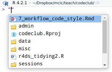
If that’s not the case, it may be easiest to copy the location using your computer’s file browser, and paste that location into your code.
Here are two examples of including folder names with a function like read_csv():
# Don't try to run this, you won't have files at these locations
# This is just meant as a general example

read_csv("data/more_students.csv")

read_csv("C:/Users/jelmer/R_data/other_students.csv")
Note that in R, you can always use forward slashes / to separate folders, regardless of your operating system (If you have Windows, which generally uses backslashes \ instead, then backslashes will also work.)
In two weeks, we’ll talk about RStudio “Projects”, which can make your life a lot easier when it comes to file paths and never having to change your working directory.
Common challenges with input files
No column names
Some files have no first line with column names. That leads to problems when using all the defaults:
read_csv("students_noheader.csv")
#> # A tibble: 5 × 5
#>     `1` `Sunil Huffmann` `Strawberry yoghurt` `Lunch only`        `4`
#>   <dbl> <chr>            <chr>                <chr>               <chr>
#> 1     2 Barclay Lynn     French fries         Lunch only          5
#> 2     3 Jayendra Lyne    N/A                  Breakfast and lunch 7
#> 3     4 Leon Rossini     Anchovies            Lunch only          NA
#> 4     5 Chidiegwu Dunkel Pizza                Breakfast and lunch five
#> 5     6 Güvenç Attila    Ice cream            Lunch only          6
Oops! The first row of data was interpreted as column names. We can tell readr to not do this by adding col_names = FALSE:
read_csv("students_noheader.csv", col_names = FALSE)
#> # A tibble: 6 × 5
#>      X1 X2               X3                 X4                  X5
#>   <dbl> <chr>            <chr>              <chr>               <chr>
#> 1     1 Sunil Huffmann   Strawberry yoghurt Lunch only          4
#> 2     2 Barclay Lynn     French fries       Lunch only          5
#> 3     3 Jayendra Lyne    N/A                Breakfast and lunch 7
#> 4     4 Leon Rossini     Anchovies          Lunch only          NA
#> 5     5 Chidiegwu Dunkel Pizza              Breakfast and lunch five
#> 6     6 Güvenç Attila    Ice cream          Lunch only          6
That’s better! But of course, we can’t automatically get useful column names, and they are now named X1, X2, etc. We could set the column names after reading the file, but we can also provide a vector of column names to the col_names argument of read_csv():
# (I am creating a vector with column names up front. But this is just for code
#  clarity -- you can also pass the names to read_csv directly.)
student_colnames <- c("student_id", "full_name", "fav_food", "meal_plan", "age")

read_csv("students_noheader.csv", col_names = student_colnames)
#> # A tibble: 6 × 5
#>   student_id full_name        fav_food           meal_plan           age
#>        <dbl> <chr>            <chr>              <chr>               <chr>
#> 1          1 Sunil Huffmann   Strawberry yoghurt Lunch only          4
#> 2          2 Barclay Lynn     French fries       Lunch only          5
#> 3          3 Jayendra Lyne    N/A                Breakfast and lunch 7
#> 4          4 Leon Rossini     Anchovies          Lunch only          NA
#> 5          5 Chidiegwu Dunkel Pizza              Breakfast and lunch five
#> 6          6 Güvenç Attila    Ice cream          Lunch only          6
Extra header or metadata lines
Other files will contain lines at the top that are not part of the table, but contain some sort of annotations or metadata, for instance:
# This file contains important information
# about some of our students
Student ID,Full Name,favourite.food,mealPlan,AGE
1,Sunil Huffmann,Strawberry yoghurt,Lunch only,4
2,Barclay Lynn,French fries,Lunch only,5
3,Jayendra Lyne,N/A,Breakfast and lunch,7
4,Leon Rossini,Anchovies,Lunch only,
5,Chidiegwu Dunkel,Pizza,Breakfast and lunch,five
6,Güvenç Attila,Ice cream,Lunch only,6
Since there are two “metadata lines”, we can tell readr to skip those first 2 lines with the skip = n argument:
read_csv("students_with_meta.csv", skip = 2)
#> # A tibble: 6 × 5
#>   `Student ID` `Full Name`      favourite.food     mealPlan            AGE
#>          <dbl> <chr>            <chr>              <chr>               <chr>
#> 1            1 Sunil Huffmann   Strawberry yoghurt Lunch only          4
#> 2            2 Barclay Lynn     French fries       Lunch only          5
#> 3            3 Jayendra Lyne    N/A                Breakfast and lunch 7
#> 4            4 Leon Rossini     Anchovies          Lunch only          NA
#> 5            5 Chidiegwu Dunkel Pizza              Breakfast and lunch five
#> 6            6 Güvenç Attila    Ice cream          Lunch only          6
Another way of skipping lines is with the comment argument, which can be used when all metadata lines start with a certain character, like # in our case:
read_csv("students_with_meta.csv", comment = "#")
#> # A tibble: 6 × 5
#>   `Student ID` `Full Name`      favourite.food     mealPlan            AGE
#>          <dbl> <chr>            <chr>              <chr>               <chr>
#> 1            1 Sunil Huffmann   Strawberry yoghurt Lunch only          4
#> 2            2 Barclay Lynn     French fries       Lunch only          5
#> 3            3 Jayendra Lyne    N/A                Breakfast and lunch 7
#> 4            4 Leon Rossini     Anchovies          Lunch only          NA
#> 5            5 Chidiegwu Dunkel Pizza              Breakfast and lunch five
#> 6            6 Güvenç Attila    Ice cream          Lunch only          6
Why might it be preferable to use comment over skip, when possible?
Missing values denotations
R has a special data type for missing values: NA. It is important for downstream analyses that missing values are actually interpreted by R as NAs.
The na argument of the readr functions controls which values are interpreted as NA. The default is to interpret empty cells and cells that only contain “NA” as NA. In R code, this default is c("", "NA"), as we can see in the read_csv() help.
However, a file sometimes use other symbols to denote missing values, such as 999, X, -, or N/A, like in the students.csv file. It turns out that our students.csv file uses empty cells and N/A (and even plain NAs…), so we’ll have to tell read_csv() about that as follows:
read_csv("students.csv", na = c("N/A", ""))
#> # A tibble: 6 × 5
#>   `Student ID` `Full Name`      favourite.food     mealPlan            AGE
#>          <dbl> <chr>            <chr>              <chr>               <chr>
#> 1            1 Sunil Huffmann   Strawberry yoghurt Lunch only          4
#> 2            2 Barclay Lynn     French fries       Lunch only          5
#> 3            3 Jayendra Lyne    NA                 Breakfast and lunch 7
#> 4            4 Leon Rossini     Anchovies          Lunch only          NA
#> 5            5 Chidiegwu Dunkel Pizza              Breakfast and lunch five
#> 6            6 Güvenç Attila    Ice cream          Lunch only          6
Compare this to the output when reading in without specifying na – pay attention the the 3rd value in the favourite.food column:
read_csv("students.csv")
#> # A tibble: 6 × 5
#>   `Student ID` `Full Name`      favourite.food     mealPlan            AGE
#>          <dbl> <chr>            <chr>              <chr>               <chr>
#> 1            1 Sunil Huffmann   Strawberry yoghurt Lunch only          4
#> 2            2 Barclay Lynn     French fries       Lunch only          5
#> 3            3 Jayendra Lyne    N/A                Breakfast and lunch 7
#> 4            4 Leon Rossini     Anchovies          Lunch only          NA
#> 5            5 Chidiegwu Dunkel Pizza              Breakfast and lunch five
#> 6            6 Güvenç Attila    Ice cream          Lunch only          6
Crappy column names
You might have noticed the backticks around Student ID and Full Name when we display the dataframe. This is because these column names contain spaces, which are allowed but quite inconvenient in R.
We could go ahead and rename columns after reading in the file, e.g.:
# You'll need to use the backticks to refer to the column name with spaces!
read_csv("students.csv") |>
  rename(student_id = `Student ID`)
#> # A tibble: 6 × 5
#>   student_id `Full Name`      favourite.food     mealPlan            AGE
#>        <dbl> <chr>            <chr>              <chr>               <chr>
#> 1          1 Sunil Huffmann   Strawberry yoghurt Lunch only          4
#> 2          2 Barclay Lynn     French fries       Lunch only          5
#> 3          3 Jayendra Lyne    N/A                Breakfast and lunch 7
#> 4          4 Leon Rossini     Anchovies          Lunch only          NA
#> 5          5 Chidiegwu Dunkel Pizza              Breakfast and lunch five
#> 6          6 Güvenç Attila    Ice cream          Lunch only          6
But the students.csv file has terribly inconsistent column name styling throughout, with favourite.food (. separating words), mealPlan (“camel case”), and AGE (all caps) as the other column names. Renaming all columns gets tedious quickly, and would in fact become a serious chore if the file had, say, 50 columns.
The really nice clean_names() function from the janitor package converts all column names to “snake case” style (all lowercase, words separated by underscores, as we saw last week):
read_csv("students.csv") |>
  janitor::clean_names()
#> # A tibble: 6 × 5
#>   student_id full_name        favourite_food     meal_plan           age
#>        <dbl> <chr>            <chr>              <chr>               <chr>
#> 1          1 Sunil Huffmann   Strawberry yoghurt Lunch only          4
#> 2          2 Barclay Lynn     French fries       Lunch only          5
#> 3          3 Jayendra Lyne    N/A                Breakfast and lunch 7
#> 4          4 Leon Rossini     Anchovies          Lunch only          NA
#> 5          5 Chidiegwu Dunkel Pizza              Breakfast and lunch five
#> 6          6 Güvenç Attila    Ice cream          Lunch only          6
The notation above with janitor:: in front of the function name is making explicit that this function is part of the janitor package; also, when we use this notation, we don’t need to have the package loaded.
Other file types
-
In the breakout rooms, you’ll practice with a TSV file: as we discussed above, these are tab-delimited. They can be read with
read_tsv(). -
For rectangular plain text files with a different delimiter than commas or tabs (e.g., spaces), you can use
read_delim()and specify the delimiter. -
Excel files can be read with the readxl package: see the bonus exercise.
-
Unstructured (non-rectangular) plain text files can be read with the base R
readLines()function. -
Sometimes you will create complex R objects that aren’t easily saved as a plain text file. These can be saved as binary (non-human readable)
.rdsfiles withwrite_rds()and read withread_rds().
Breakout rooms
If you haven’t done so already, please download the CSV and TSV files and make sure you have janitor installed (see the code in the Introduction).
Exercise 1: A TSV file
Let’s try read_csv()’s counterpart for TSV (tab-separated) files: read_tsv().
The students.tsv file that you have downloaded contains the exact same data as the students.csv file we’ve practiced with.
Read in students.tsv, making sure to get the NAs right, and to clean up the column names like we did above.
Solution(click here)
-
Since missing values are represented both as “N/A” and empty cells (""), we’ll use
na = c("N/A", ""). -
We pipe the output to the
clean_names()function to get consistently “snake case”-styled column names.
read_tsv("students.tsv", na = c("N/A", "")) |>
  janitor::clean_names()
#> Rows: 6 Columns: 5
#> ── Column specification ────────────────────────────────────────────────────────
#> Delimiter: "\t"
#> chr (4): Full Name, favourite.food, mealPlan, AGE
#> dbl (1): Student ID
#>
#> ℹ Use `spec()` to retrieve the full column specification for this data.
#> ℹ Specify the column types or set `show_col_types = FALSE` to quiet this message.#> # A tibble: 6 × 5
#>   student_id full_name        favourite_food     meal_plan           age
#>        <dbl> <chr>            <chr>              <chr>               <chr>
#> 1          1 Sunil Huffmann   Strawberry yoghurt Lunch only          4
#> 2          2 Barclay Lynn     French fries       Lunch only          5
#> 3          3 Jayendra Lyne    NA                 Breakfast and lunch 7
#> 4          4 Leon Rossini     Anchovies          Lunch only          NA
#> 5          5 Chidiegwu Dunkel Pizza              Breakfast and lunch five
#> 6          6 Güvenç Attila    Ice cream          Lunch only          6
Exercise 2: A challenging file
Start by downloading the following CSV file:
url_tsv <- "https://github.com/biodash/biodash.github.io/raw/master/content/codeclub/S05E05/exercise2.csv"
download.file(url = url_tsv, destfile = "exercise2.csv")
Now, try reading in this exercise2.csv file, which has the following content:
# This file is still incomplete
1,Sunil Huffmann,Strawberry yoghurt,Lunch only,4
2,Barclay Lynn,French fries,Lunch only,5
3,Jayendra Lyne,N/A,Breakfast and lunch,7
4,Leon Rossini,Anchovies,Lunch only,
5,Chidiegwu Dunkel,Pizza,Breakfast and lunch,five
6,Güvenç Attila,Ice cream,Lunch only,6
% More data will be entered soon!
Hints(click here)
-
Notice that there are metadata / comment lines both at the start and the end of the file!
-
The
commentargument also works for lines that aren’t at the top of the file. -
But you cannot specify multiple
commentsymbols toread_csv(), so you’ll have to use both theskipandcommentarguments. -
You’ll also want to take care of the fact that there is no line with column names.
Solution(click here)
-
We’ll take care of ignoring the first metadata line with
skip = 1, and the trailing line withcomment = %since that line starts with a%. -
We use
col_names = FALSEto make sure the first row of data does not get wrongly interpreted as column names
read_csv("exercise2.csv", skip = 1, comment = "%", col_names = FALSE)
#> Rows: 6 Columns: 5
#> ── Column specification ────────────────────────────────────────────────────────
#> Delimiter: ","
#> chr (4): X2, X3, X4, X5
#> dbl (1): X1
#>
#> ℹ Use `spec()` to retrieve the full column specification for this data.
#> ℹ Specify the column types or set `show_col_types = FALSE` to quiet this message.#> # A tibble: 6 × 5
#>      X1 X2               X3                 X4                  X5
#>   <dbl> <chr>            <chr>              <chr>               <chr>
#> 1     1 Sunil Huffmann   Strawberry yoghurt Lunch only          4
#> 2     2 Barclay Lynn     French fries       Lunch only          5
#> 3     3 Jayendra Lyne    N/A                Breakfast and lunch 7
#> 4     4 Leon Rossini     Anchovies          Lunch only          NA
#> 5     5 Chidiegwu Dunkel Pizza              Breakfast and lunch five
#> 6     6 Güvenç Attila    Ice cream          Lunch only          6
The code above resulted in column names like X1 and X2. To get descriptive column names, we’ll have to write a vector with such names, and pass those to col_names =:
student_colnames <- c("student_id", "full_name", "fav_food", "meal_plan", "age")

read_csv("exercise2.csv", skip = 1, comment = "%", col_names = student_colnames)
#> Rows: 6 Columns: 5
#> ── Column specification ────────────────────────────────────────────────────────
#> Delimiter: ","
#> chr (4): full_name, fav_food, meal_plan, age
#> dbl (1): student_id
#>
#> ℹ Use `spec()` to retrieve the full column specification for this data.
#> ℹ Specify the column types or set `show_col_types = FALSE` to quiet this message.#> # A tibble: 6 × 5
#>   student_id full_name        fav_food           meal_plan           age
#>        <dbl> <chr>            <chr>              <chr>               <chr>
#> 1          1 Sunil Huffmann   Strawberry yoghurt Lunch only          4
#> 2          2 Barclay Lynn     French fries       Lunch only          5
#> 3          3 Jayendra Lyne    N/A                Breakfast and lunch 7
#> 4          4 Leon Rossini     Anchovies          Lunch only          NA
#> 5          5 Chidiegwu Dunkel Pizza              Breakfast and lunch five
#> 6          6 Güvenç Attila    Ice cream          Lunch only          6
Bonus: reading an Excel file
In this exercise, you’ll use a function from the readxl package to read an Excel file. We need to do a couple of things to get set up first.
- You can install and then load the readxl package as follows:
install.packages("readxl")- You can download the excel file as follows:
url_xls <- "https://github.com/biodash/biodash.github.io/raw/master/content/codeclub/S05E05/breed_ranks.xlsx"
download.file(url = url_xls, destfile = "breed_ranks.xlsx")
Now, use the read_excel() function from the readxl package to read the breed_ranks.xlsx file.
Bonus2: There are two sheets in the Excel file: Sheet1 and Sheet2. Can you read both in? And can you combine the resulting dataframes into a single one?
Hints(click here)
-
Take a look at the
read_excel()help page (e.g., type?read_excelin the R console) to figure out the syntax. -
When you don’t specify the
sheetargument, it will read in the first one. -
You can “vertically” combine dataframes using the
bind_rows()function.
Solution(click here)
read_excel will by default read the first sheet of an Excel file, so you can read the first sheet simply with:
breed_ranks <- read_excel("breed_ranks.xlsx")

# Or, equivalently:
#breed_ranks <- read_excel("breed_ranks.xlsx", sheet = 1)
You can read the second sheet by using the sheet = argument:
breed_ranks2 <- read_excel("breed_ranks.xlsx", sheet = 2)You can combine the two dataframes with the bind_rows() function, which will simply “row-bind” (vertically paste, or “concatenate”) the two files:
breed_ranks_all <- bind_rows(breed_ranks, breed_ranks2)(The base R function rbind() would also work.)
Let’s check the numbers of rows to check that our row-binding was successful:
nrow(breed_ranks) # From sheet 1
#> [1] 100
nrow(breed_ranks2) # From sheet 2
#> [1] 94
nrow(breed_ranks_all) # Both combined
#> [1] 194
Let’s also take a look at the first few rows of the dataframe:
head(breed_ranks_all)
#> # A tibble: 6 × 22
#> Breed 2013 …¹ 2014 …² 2015 …³ 2016 …⁴ 2017 …⁵ 2018 …⁶ 2019 …⁷ 2020 …⁸ links
#> <chr> <chr> <chr> <chr> <chr> <chr> <chr> <chr> <dbl> <chr>
#> 1 Retriev… 1 1 1 1 1 1 1 1 http…
#> 2 French … 11 9 6 6 4 4 4 2 http…
#> 3 German … 2 2 2 2 2 2 2 3 http…
#> 4 Retriev… 3 3 3 3 3 3 3 4 http…
#> 5 Bulldogs 5 4 4 4 5 5 5 5 http…
#> 6 Poodles 8 7 8 7 7 7 6 6 http…
#> # … with 12 more variables: Image <chr>, `Setters (English)` <chr>, `91` <chr>,
#> # `89` <chr>, `96` <chr>, `102` <chr>, `95` <chr>, `94` <chr>, `100` <chr>,
#> # `101` <dbl>, `https://www.akc.org/dog-breeds/english-setter/` <chr>,
#> # `https://www.akc.org/wp-content/uploads/2017/11/English-Setter-Illo-2.jpg` <chr>,
#> # and abbreviated variable names ¹`2013 Rank`, ²`2014 Rank`, ³`2015 Rank`,
#> # ⁴`2016 Rank`, ⁵`2017 Rank`, ⁶`2018 Rank`, ⁷`2019 Rank`, ⁸`2020 Rank`