S05E01: R for Data Science (2e) - Ch. 5 - Pipes
Introducing a new season of Code Club, in which we will continue to read the book R for Data Science (R4DS), and start with a short chapter on pipes.
Intro to this Code Club Season
Organizers
- Michael Broe – Evolution, Ecology and Organismal Biology (EEOB)
- Jessica Cooperstone – Horticulture & Crop Science (HCS) / Food Science & Technology (FST)
- Stephen Opiyo – Molecular & Cellular Imaging Center (MCIC) - Columbus
- Jelmer Poelstra – Molecular & Cellular Imaging Center (MCIC) - Wooster
Code Club practicalities
-
In-person (Columbus & Wooster) and Zoom hybrid
-
Mix of instruction/discussion with the entire group, and exercises in groups of 3-4 people.
-
When doing exercises in breakout groups, we encourage you:
- To briefly introduce yourselves and to do the exercises as a group
- On Zoom, to turn your cameras on and to have someone share their screen (use the
Ask for helpbutton in Zoom to get help from an organizer) - To let a less experienced person do the screen sharing and coding
-
You can ask a question at any time, by speaking or typing in the Zoom chat.
-
You can come up to 15 minutes early or stay late for troubleshooting and perhaps a question related to your research.
More general notes:
-
If you can, read or skim the relevant (part of the) chapter before each session, especially if you’re very new to the material. But we’ll always try to present it in such a way that does not assume you’ve read it.
-
We try to make each session as stand-alone as possible, and don’t require you to know anything. That said, if you missed one or more sessions, you’ll get more out of the next ones if you try to catch up with the material.
-
We record the whole-group parts of the Zoom call, and share the recordings only with Code Club participants.
New to Code Club or R?
Take a look at these pages on our website:
Before moving on the the chapter on pipes, I will start with a very brief overview of the book, the RStudio interface, and how to load R packages.
R for Data Science (R4DS)
This excellent book by Hadley Wickham (also author of many of the R packages used in the book!) and Garret Grolemund is freely available online.
The book focuses on the so-called "tidyverse" ecosystem in R. The tidyverse can be seen as a modern dialect of R. Most of its functionality is also contained in “base R” (that which comes shipped with R by default), but it has an improved and more consistent programming interface or “syntax”.
Last year in Code Club, we worked through the material of a number of chapters of the first edition of the book, which was published in 2016.
Since 2016, quite some R development has taken place. A second edition has been online since a couple of months, with completely updated and also restructured contents – we thought it has improved a lot!
This new edition is not completely finished yet, so you’ll find notifications like these at the top of each chapter:
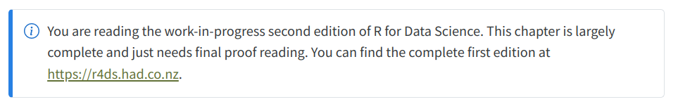
We decided not to restart at the beginning of the book for this semester. We hope this won’t make it too challenging for beginners to join us. Especially in the first sessions, we’ll make sure to explain all code, including things that were covered last semester.
What’s in the book
The introductory chapter of the book has this figure to show the data science process and what the book will cover:

In terms of what the book does not cover, it may especially be surprising for a book about data science that it contains very little material on statistics (even less so in the second edition, now that there is a companion book “Tidy Modeling with R” on that topic).
Getting Up and Running
RStudio interface
R itself simply provides a “console” (command-line interface) where you can type your commands. RStudio, on the other hand, allows you to see the R console side-by-side with your scripts, plots, and more.
Once you have a running instance of RStudio, create a new R script by clicking File > New File > R Script. Now, you should see all 4 “panes” that the RStudio window is divided into:
- Top-left: The Editor for your scripts and other documents (hidden when no file is open)
- Bottom-left: The R Console to interactively run your code (+ other tabs)
- Top-right: Your Environment with R objects you have created (+ other tabs)
- Bottom-right: Tabs for Files, Plots, Help, and others

Your turn: Check your R version
Take a look at your version of R: this was printed in the console when you started RStudio (see the RStudio screenshot above).
The most recent version of R is 4.2.2. To use all current functionality of the “base R pipe”, you’ll need at least version 4.2.0, and to use the base R pipe at all, you need at least R version 4.1.
If you have a lower version of R, I would recommend that you update at the end or after this session following these instructions.
R packages
You can think of packages as “add-ons” / “extensions” to base R functionality.
Installation versus loading
To be able to use them, packages have to be installed (usually from within R, using R code). Once you have done this, you don’t need to redo it until you switch to a different version of R.
Unlike installation, loading a package is necessary again and again, in every R session that you want to use it.
The tidyverse
The tidyverse is unusual in that it is a collection of packages that can still be installed and loaded with a single command. The individual core tidyverse packages are the focus of several chapters in the book, for instance:
| Package | Functionality | Main chapter |
|---|---|---|
| ggplot2 | Creating plots | Ch. 2 |
| tidyr & dplyr | Manipulating dataframes | Ch. 4 & 6 |
| readr | Reading in data | Ch. 8 |
| stringr | Working with “strings” (text) | Ch. 16 |
| forcats | Working with “factors” (categorical variables) |
Ch. 18 |
| purrr | Iteration with functions | Ch. 28 |
Your turn: Load the tidyverse
To check if you can load the tidyverse, run the following and see if you get similar output as printed below:

If instead, you got something like…
#> Error in library(tidyverse) : there is no package called ‘tidyverse’…then you still need to install it (install.packages("tidyverse")).
The diamonds dataframe
In R, we work a lot with “dataframes”, rectangular data structures like spreadsheets – and in particular, the R4DS book and the tidyverse focus on this very heavily.
Today we’ll see some examples of using the pipe with the diamonds dataframe, which is automatically loaded along with the tidyverse. It contains information on almost 54,000 diamonds (one diamond per row):
# Simply typing the dataframe's name in the console will print the first rows:
diamonds
#> # A tibble: 53,940 × 10
#>    carat cut       color clarity depth table price     x     y     z
#>    <dbl> <ord>     <ord> <ord>   <dbl> <dbl> <int> <dbl> <dbl> <dbl>
#>  1  0.23 Ideal     E     SI2      61.5    55   326  3.95  3.98  2.43
#>  2  0.21 Premium   E     SI1      59.8    61   326  3.89  3.84  2.31
#>  3  0.23 Good      E     VS1      56.9    65   327  4.05  4.07  2.31
#>  4  0.29 Premium   I     VS2      62.4    58   334  4.2   4.23  2.63
#>  5  0.31 Good      J     SI2      63.3    58   335  4.34  4.35  2.75
#>  6  0.24 Very Good J     VVS2     62.8    57   336  3.94  3.96  2.48
#>  7  0.24 Very Good I     VVS1     62.3    57   336  3.95  3.98  2.47
#>  8  0.26 Very Good H     SI1      61.9    55   337  4.07  4.11  2.53
#>  9  0.22 Fair      E     VS2      65.1    61   337  3.87  3.78  2.49
#> 10  0.23 Very Good H     VS1      59.4    61   338  4     4.05  2.39
#> # … with 53,930 more rows
(If you get Error: object 'diamonds' not found, then the tidyverse isn’t loaded. Use library(tidyverse) to do so.)
Chapter 5: Pipes
What is a pipe?
A pipe is a programming tool that takes the output of one command (in R, a function), and passes it on to be used as the input for another command.
Pipes prevent you from having to save intermediate output to a file or object. They also make your code shorter and easier to understand.
To give a very minimal example – without a pipe, we can print the number of rows in the diamonds dataframe as follows:
# Use the `nrow()` function with `diamonds` as the sole argument:
nrow(diamonds)
#> [1] 53940
Instead, we could also take the diamonds dataframe, and then pipe (|>) it into the nrow() function:
diamonds |> nrow()
#> [1] 53940
Notice above that we no longer type the input argument to nrow() inside the parentheses: nrow() recognizes that data came in through the pipe.
A more practical example
Let’s say we want to subset the diamonds dataframe to only show the columns color, depth, and price for diamonds with a depth smaller than 50. Without using pipes, we could start by selecting the columns of interest with the select() function, and saving the output in a new dataframe called diamonds_simple:
# The first argument is the input dataframe, the others are the columns we want
diamonds_simple <- select(diamonds, color, depth, price)
Next, we can use the filter() function on diamonds_simple to only return the diamonds (rows) that we want:
# The first argument is the input dataframe, the next is an expression to filter by
filter(diamonds_simple, depth < 50)
#> # A tibble: 3 × 3
#>   color depth price
#>   <ord> <dbl> <int>
#> 1 G        43  3634
#> 2 G        44  4032
#> 3 J        43  4778
But using the pipe, we can do this more elegantly, and without wasting computer memory on an intermediate object:
diamonds |>                       # Take 'diamonds' and push it through the pipe
  select(color, depth, price) |>  # No input is specified, and the output is piped
  filter(depth < 50)              # Again, no input is specified
#> # A tibble: 3 × 3
#>   color depth price
#>   <ord> <dbl> <int>
#> 1 G        43  3634
#> 2 G        44  4032
#> 3 J        43  4778
We took the diamonds dataset and piped it into the select() function, and then we piped the output of select() into the filter() function. Using the the pipe before select() is not necessary and adds a line, but also makes it even easier to see what’s being done!
Like in the earlier example, when we use the pipe, we don’t type the corresponding input argument in the receiving function: it knows to use the piped data. This is not completely “automagical” and foolproof though: what actually happens is that the piped data becomes the first argument to the receiving function.
If you ever need to use the pipe with a function where the piped data is not the first argument, see the Bonus section below about using the _ placeholder.
Two Unix & R examples
Pipes originate in Unix terminals, and are ubiquitous there. So for those of you that are curious, I’ve included two examples of using the Unix pipe, and the corresponding commands in R, in the dropdown box below.
See the examples (click here)
(If you’re trying to follow along yourself: the Unix/terminal examples will only work natively on Mac and Linux, where you can simply click the Terminal tab in the bottom-left RStudio panel next to Console, and issue Unix commands.)
Counting files
You might want to count the number of files in a folder, which involve two distinct processes: obtaining a list of files, and counting them.
Using Unix commands, We can get a list of files in the current folder with ls, perform the counting with wc -l (wordcount -lines), and connect these processes with the pipe |:
# The output of 'ls' is piped (with '|') to 'wc -l':
ls | wc -l


#> 4
So, there happen to be 4 files in the folder this code is run in. We can do the same in R, where the function dir() lists files, while the function length() counts the number of elements:
Counting word frequencies
As another example, let’s say we have a file words.txt that contains one word per line:
table
chair
desk
chair
desk
table
chair
In a terminal, we can get a list of unique words and their number of occurrences using:
# 'cat' prints the contents of the file
# 'sort' sorts alphabetically
# 'uniq -c' counts the number of occurrences for each entry
cat words.txt | sort | uniq -c


#>       3 chair
#>       2 desk
#>       2 table
And to do the same thing in R:
The %>% pipe and a keyboard shortcut
Those of you who’ve worked with R for a bit are likely familiar with another pipe operator: %>%.
This pipe is loaded as part of the tidyverse, and until recently was very widely used, including in the previous edition of R4DS. There has been a gradual switch to the base R pipe since that was introduced in May 2021, mainly because it does not rely on a package. In addition, it’s convenient that the base R pipe |> is more similar to the Unix pipe |, and is one fewer character to type than %>%.
The number of characters shouldn’t make much of a difference, though, because it remains even quicker to use the RStudio keyboard shortcut for the pipe, which is Ctrl+Shift+M.
There are some differences in the behavior of the |> and %>% pipes in more advanced use cases, which the book chapter goes into (check that out if you have used %>% a lot).
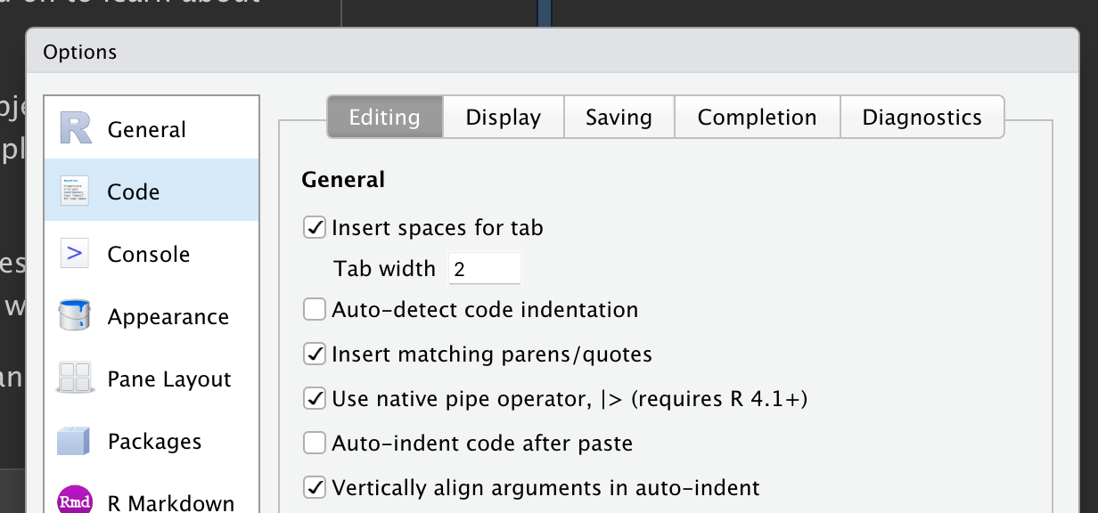
Your turn: Set the |> pipe as default
To make that keyboard shortcut map to the base R pipe (instead of to %>%), go to Tools in the top menu bar, click Global Options, click Code in the left menu, and check the box Use native pipe operator, |> (requires R 4.1+):
Your turn: Use the pipe
With one single “pipeline” (operations connected by a pipe |>), manipulate the diamonds dataframe such that you:
- Print only the columns
carat,cut,depth, andprice - … for diamonds (rows) with a
priceof more than $1,000.
Bonus: How many diamonds cost more than $1,000? And could you get this number directly, by expanding your “pipeline”?
Hints(click here)
This is quite similar to the example given above: use the select() function to select certain columns, and the filter() function to select certain rows.
To answer the bonus question: each diamond is on one row, so you are counting rows. And to answer it by expanding your pipeline, recall from the very first pipe example that the nrow() function will print the number of rows.
Solution(click here)
diamonds |>
  select(carat, cut, depth, price) |>
  filter(price > 1000)
#> # A tibble: 39,416 × 4
#>    carat cut       depth price
#>    <dbl> <ord>     <dbl> <int>
#>  1  0.7  Ideal      62.5  2757
#>  2  0.86 Fair       55.1  2757
#>  3  0.7  Ideal      61.6  2757
#>  4  0.71 Very Good  62.4  2759
#>  5  0.78 Very Good  63.8  2759
#>  6  0.7  Good       57.5  2759
#>  7  0.7  Good       59.4  2759
#>  8  0.96 Fair       66.3  2759
#>  9  0.73 Very Good  61.6  2760
#> 10  0.8  Premium    61.5  2760
#> # … with 39,406 more rows
10 rows are printed to screen, and it says … with 39,406 more rows at the bottom: therefore, there are 39,416 diamonds that cost more than $1,000.
You can also get this number with code – for instance by adding the nrow() function to the pipeline, which will count the number of rows (excluding the header line) in a dataframe:
Bonus: Using the _ placeholder
By default, the R pipe passes its contents to the first argument of a function. What if we need our piped data to go to another argument than the function’s first one?
Let’s see an example with the gsub() function, which can be used to replace characters in text strings as follows:
# This will replace 'N's with '-' in the string 'ACCGNNT':
gsub(pattern = "N", replacement = "-", x = "ACCGNNT")
#> [1] "ACCG--T"
(For clarity, I named gsub()’s arguments above. Without naming the arguments, it would be: gsub("N", "-", "ACCGNNT")).
As you could see above, what we would usually think of as the input data, the string passed to the argument x, is not the first but the third argument to gsub().
To make the pipe work with gsub(), use an underscore (_) as a placeholder that indicates where the piped data goes:
"ACCGNNT" |> gsub(pattern = "N", replacement = "-", x = _)
#> [1] "ACCG--T"
As an aside, if you’re wondering how you’d know a function’s argument order, watch the pop-up box when you type a function’s name and the opening parenthesis (see the screenshot below), or check the help e.g. by typing ?gsub in the Console.

Above, I mentioned that the pipe passes its contents to the first argument of a function. But to be more precise, the pipe passes the object to the first argument that you didn’t mention by name. Therefore, the following also works:
# The piped data is being passed to the 3rd argument, 'x',
# which is the first of the function's arguments that we don't refer to below:
"ACCGNNT" |> gsub(pattern = "N", replacement = "-")
#> [1] "ACCG--T"
Additionally, when you do use the _ placeholder, make sure you always name the argument that you pass it to:
# Using '_' without the argument name ('x=') doesn't work:
"ACCGNNT" |> gsub(pattern = "N", replacement = "-", _)

#> Error: pipe placeholder can only be used as a named argument