S04E09: R for Data Science - Chapter 5.1 - 5.2

I – Chapter 5.1: Introduction

Key points

• Function name conflicts: The function filter() in the stats package (which is loaded by default in R) will be “masked” / “overwritten” by dplyr’s filter() function when you load the tidyverse. To still use a masked function (or a function from an installed-but-not-loaded package!), use the “full” notation, e.g. stats::filter().

• A data frame is rectangular data structure (with rows and columns), while a “tibble” is a tidyverse-style data frame. Tibbles mainly differ from regular data frames in how they are printed to screen by default. See the two examples below: cars is a regular data frame and flights is a tibble.

• The most common R data types are integers (tibble abbreviation: int), doubles (dbl), character strings (chr), logicals (lgl), and factors (fctr).

• The dplyr package is designed to work with dataframes: both the input and the output is a dataframe.

# 'mtcars' is a regular dataframe
head(mtcars)

#>                    mpg cyl disp  hp drat    wt  qsec vs am gear carb
#> Mazda RX4         21.0   6  160 110 3.90 2.620 16.46  0  1    4    4
#> Mazda RX4 Wag     21.0   6  160 110 3.90 2.875 17.02  0  1    4    4
#> Datsun 710        22.8   4  108  93 3.85 2.320 18.61  1  1    4    1
#> Hornet 4 Drive    21.4   6  258 110 3.08 3.215 19.44  1  0    3    1
#> Hornet Sportabout 18.7   8  360 175 3.15 3.440 17.02  0  0    3    2
#> Valiant           18.1   6  225 105 2.76 3.460 20.22  1  0    3    1

# 'flights' is a tibble, which affects its printing behavior
library(nycflights13)
head(flights)

#> # A tibble: 6 × 19
#>    year month   day dep_time sched_dep…¹ dep_d…² arr_t…³ sched…⁴ arr_d…⁵ carrier
#>   <int> <int> <int>    <int>       <int>   <dbl>   <int>   <int>   <dbl> <chr>  
#> 1  2013     1     1      517         515       2     830     819      11 UA     
#> 2  2013     1     1      533         529       4     850     830      20 UA     
#> 3  2013     1     1      542         540       2     923     850      33 AA     
#> 4  2013     1     1      544         545      -1    1004    1022     -18 B6     
#> 5  2013     1     1      554         600      -6     812     837     -25 DL     
#> 6  2013     1     1      554         558      -4     740     728      12 UA     
#> # … with 9 more variables: flight <int>, tailnum <chr>, origin <chr>,
#> #   dest <chr>, air_time <dbl>, distance <dbl>, hour <dbl>, minute <dbl>,
#> #   time_hour <dttm>, and abbreviated variable names ¹​sched_dep_time,
#> #   ²​dep_delay, ³​arr_time, ⁴​sched_arr_time, ⁵​arr_delay

II – Chapter 5.2: filter()

Key points

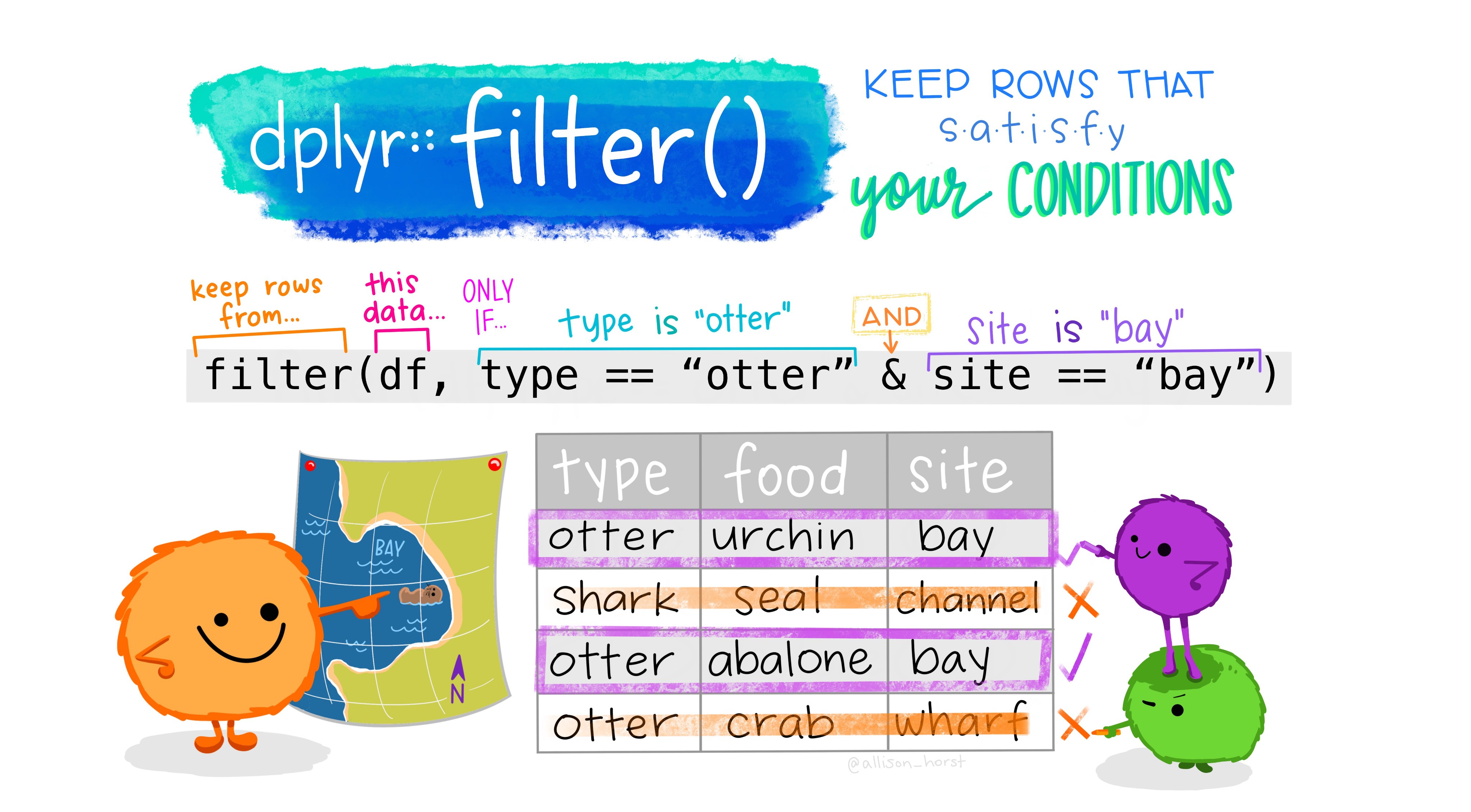
• The filter() function removes rows (observations) from a dataframe based on certain conditions. You specify those conditions for one or more columns.

• When you refer to a column, don’t quote its name! (e.g. in filter(flights, month == 1), where month is the column name.)

• Use “comparison operators” like > (greater than) to specify conditions. Note that two equals signs == (and not a single, =) signifies equality, and that != means “does not equal”.

• To combine multiple conditions, use logical (Boolean) operators: & (and), | (or), and ! (not). Separating conditions by a comma also means “and” in dplyr, e.g. in filter(flights, month == 1, day == 1).

• The %in% operator tests if the value(s) on the left-hand side are contained in the values on the right hand side, e.g. 4 %in% 1:5 asks whether 4 is contained in the sequence of numbers from 1 to 5, which will return TRUE.

• Missing values are denoted by NA, and almost any operation with an NA will return another NA. To test if x is or contains NAs, don’t use x == NA but is.na(x). When you filter based on a column, rows with NAs in that column will by default be removed by filter().

library(nycflights13)
library(tidyverse)

filter(flights,
       arr_delay >= 120) %>%
  nrow()

#> [1] 10200

filter(flights,
       dest %in% c("IAH", "HOU")) %>%
  nrow()

#> [1] 9313

filter(flights,
       carrier %in% c("UA", "AA", "DL")) %>%
  nrow()

#> [1] 139504

filter(flights,
       month %in% 7:9) %>%
  nrow()

#> [1] 86326

filter(flights,
       month >= 7, month <= 9) %>%
  nrow()

filter(flights,
       arr_delay > 120, dep_delay <= 0) %>%
  nrow()

#> [1] 29

filter(flights,
       dep_delay >= 60, dep_delay - arr_delay > 30) %>%
  nrow()

#> [1] 1844

filter(flights,
       dep_time <= 600 | dep_time == 2400) %>%
  nrow()

#> [1] 9373

filter(flights,
       is.na(dep_time)) %>%
  nrow()

#> [1] 8255