S04E01: R for Data Science - Chapter 1
Introducing a new season of Code Club, in which we will read the book R for Data Science (R4DS)

I – Intro to this season of Code Club
Organizers
- Michael Broe – Evolution, Ecology and Organismal Biology (EEOB)
- Jessica Cooperstone – Horticulture & Crop Science (HCS) / Food Science & Technology (FST)
- Stephen Opiyo – Molecular & Cellular Imaging Center (MCIC) - Columbus
- Jelmer Poelstra – Molecular & Cellular Imaging Center (MCIC) - Wooster
- Mike Sovic – Center for Applied Plant Sciences (CAPS)
Code Club practicalities
-
In-person (Columbus & Wooster) and Zoom hybrid
-
Mix of instruction/discussion with the entire group, and doing exercises in breakout groups of up to 4-5 people.
-
When doing exercises in breakout groups, we encourage you:
- To briefly introduce yourselves and to do the exercises as a group
- On Zoom, to turn your cameras on and to have someone share their screen (use the
Ask for helpbutton in Zoom to get help from an organizer) - To let a less experienced person do the screen sharing and coding
-
You can ask a question at any time, by speaking or typing in the Zoom chat.
-
You can generally come early or stay late for troubleshooting but also for questions related to your research.
More general notes:
-
We recommend that you read the relevant (part of the) chapter before each session, especially if the material in the chapter is new to you.
-
We try to make each session as stand-alone as possible. Still, if you missed one or more sessions, you would ideally catch up on reading those parts of the book, especially when we split a chapter across multiple sessions.
-
We record the whole-group parts of the Zoom call, and share the recordings only with Code Club participants.
-
We’re always hoping for someone outside of the group of organizers to lead a session – this might be more feasible now that we’re going through a book?
New to Code Club or R?
Take a look at these pages on our website:
- Computer setup for Code Club
- Resources and tips to get started with R
- List of all previous Code Club session topics
II – The R for Data Science book (R4DS)
This excellent book by Hadley Wickham (also author of many of the R packages used in the book!) and Garret Grolemund, has a freely available online version that is regularly updated and contains exercises. It was originally published in 2016.
The book focuses on the so-called "tidyverse" ecosystem in R. The tidyverse can be seen as a modern dialect of R. Most of its functionality is also contained in “base R” (that which comes shipped with R by default), but it has an improved and more consistent programming interface or “syntax”. In previous Code Clubs, we have often –but not always!– been doing things “the tidyverse way” as well.
The book doesn’t technically assume any previous experience with R, but if you’re completely new to R and to coding in any language, we would recommend you take a look at some introductory R material (see this page for some resources) before we start with Chapter 2 next week.
We will not be able to finish the book by the end of the summer. But if folks are liking the book, we may carry on with it during the fall semester.
III – R4DS Chapter 1 notes
1.1 - What you will learn
The data science process visualized:

What is tidy data?
Brief explanation and examples (Click here)
First, you can think of this along the lines of the colloquial meaning of the word: the data is well-organized.
Additionally, computer-readability should be prioritized over human-readability (think: no color-coded cells, multiple header columns, or merged cells).
But, most of all, “tidy” in the context of the tidyverse refers to the following, as it is phrased in the book:
In brief, when your data is tidy, each column is a variable, and each row is an observation.
But what does this mean? In practice, it often means having your data not in a “wide format” (all the information about each sample/individual in one row) but in a “long format” (variables not spread across multiple columns) – see the examples below.
Example 1, not tidy:
#>     name quiz1 quiz2 test1
#> 1  Billy     C     D     C
#> 2   Suzy     F     A     A
#> 3 Lionel     B     C     B
Example 1, tidy:
#> # A tibble: 9 × 3
#>   name   assessment grade
#>   <chr>  <chr>      <chr>
#> 1 Billy  quiz1      C
#> 2 Billy  quiz2      D
#> 3 Billy  test1      C
#> 4 Lionel quiz1      B
#> 5 Lionel quiz2      C
#> 6 Lionel test1      B
#> 7 Suzy   quiz1      F
#> 8 Suzy   quiz2      A
#> 9 Suzy   test1      A
Example 2, not tidy (in matrix form):
#>         gene1 gene2 gene3 gene4 gene5
#> sample1    48    53    42    50    52
#> sample2    39    43    37    64    47
#> sample3    45    55    51    58    52
#> sample4    42    40    41    64    49
#> sample5    48    49    54    49    43
Example 2, tidy:
#> # A tibble: 25 × 3
#>    sample  gene  count
#>    <chr>   <chr> <int>
#>  1 sample1 gene1    48
#>  2 sample1 gene2    53
#>  3 sample1 gene3    42
#>  4 sample1 gene4    50
#>  5 sample1 gene5    52
#>  6 sample2 gene1    39
#>  7 sample2 gene2    43
#>  8 sample2 gene3    37
#>  9 sample2 gene4    64
#> 10 sample2 gene5    47
#> # … with 15 more rows
The tidyverse is, as the name suggests, generally designed to work with data that is “tidy” as shown above. With ggplot2, in particular, you’ll quickly run into difficulties when trying to make plots using wide-format dataframes.
For more, the book has a separate chapter on tidy data, and there is also tidyr package explainer on tidy data.
1.3 - What you won’t learn
Some perhaps unfamiliar terms from this section:
1.3.1 - Processing big data
Fortunately each problem is independent of the others (a setup that is sometimes called embarrassingly parallel), so you just need a system (like Hadoop or Spark) that allows you to send different datasets to different computers for processing.
At OSU, and most other universities, we instead tend to make use of “supercomputers” when we want to simultaneously run an analysis many times, and more broadly, if we have “big data”. Specifically, we have the “Ohio Supercomputer Center” (OSC) here.
1.3.3 - Non-rectangular data
Rectangular data is basically data that can be effectively entered in a spreadsheet (and in R, we tend to put this in a so-called “dataframe” or “tibble”). The tidyverse is highly dataframe-oriented, so it makes sense that the book focuses on rectangular data.
1.4.2 - RStudio interface
R itself simply provides a “console” (command-line interface) where you can type your commands. RStudio, on the other hand, allows you to see the R console side-by-side with your scripts, plots, and more.
Once you have a running instance of RStudio, create a new R script by clicking File > New File > R Script. Now, you should see all 4 “panes” that the RStudio window is divided into:
- Top-left: The Editor for your scripts and other documents (hidden when no file is open).
- Bottom-left: The R Console to interactively run your code (+ other tabs).
- Top-right: Your Environment with R objects you have created (+ other tabs).
- Bottom-right: Tabs for Files, Plots, Help, and others.

Check that you have R and RStudio working
Take a moment to explore the RStudio interface. Were you able to open a new file to get the Editor pane?
Take a look at your version of R: this was printed in the console when you started RStudio (see the RStudio screenshot above).
The current version of R is 4.2.0. If your version of R is below 4.0, it will be a good idea to update R. To do so, you can follow these instructions. But it is better to start this process at the very end of this session or after it, since it may take a while.
1.4.3 & 1.4.4 - R packages
An R package is a collection of functions, data, and documentation that extends the capabilities of base R.
So, you can think of packages as “add-ons” / “extensions” to base R.
Installation versus loading
Packages have to be separately installed (usually from within R, using R code) and once you have done this, you don’t need to redo it unless:
- You want a different version of the package
- You have switched to a different version of R
Unlike installation, loading a package is necessary again and again, in every R session that you want to use it.
The tidyverse
The tidyverse is unusual in that it is a collection of packages that can still be installed and loaded with a single command. The individual tidyverse packages are the focus of several chapters in the book, for instance:
| Package | Functionality | Main chapter |
|---|---|---|
| ggplot2 | Creating plots | Ch. 3 |
| tidyr & dplyr | Manipulating dataframes | Ch. 5 & 7 |
| readr | Reading in data | Ch. 11 |
| stringr | Working with “strings” (text) | Ch. 14 |
| forcats | Working with “factors” (categorical variables) |
Ch. 15 |
| purrr | Iteration with functions | Ch. 21 |
Data packages
Additionally, the book uses a couple of “data packages” (packages that only contain data, and no functions): nycflights13, gapminder, and Lahman.
IV – Breakout rooms
1. Introduce yourselves!
Please take a moment to introduce yourself to your breakout roommates. You may also want to mention:
-
Your level of experience with R (and perhaps other coding languages)
-
What you want to use R for, or what you are already using R for
-
Why you think this book might be useful, if you have an idea already
2. Install/load the packages
Usually, exercises can be done with your breakout group on one computer, but the following should be done individually, to check that everyone has R up and running.
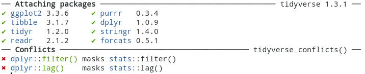
Most of you should already have the tidyverse installed, so let’s start by trying to load it. This is done with the library() function. To check if you can load the tidyverse, run the following and see if you get similar output as printed below:
If instead, you got something like:
#> Error in library(tidyverse) : there is no package called ‘tidyverse’…that means you still need to install it:
## Note: the package name is "quoted" in the install.packages() function:
install.packages("tidyverse")

## ... but it is not (normally) in library():
library(tidyverse)
Now, let’s also install the data packages – we can do that all at once:
install.packages(c("nycflights13", "gapminder", "Lahman"))The previous installation commands should return a whole bunch of output, but if all went well, you should not see any errors. Instead, look for phrases like * DONE (nycflights13), which indicate successful installation of a package.
You can also load the data packages (we have to do that for each package individually):
You won’t see any output when loading most packages, like the three above (but unlike the tidyverse).
Bonus question: What are these “conflicts” in the tidyverse startup messages referring to?
3. Bonus: Questions or remarks about the chapter?
Discuss or ask about whatever you thought was interesting/confusing/etc about the chapter!
If nothing else comes up, you could think about and discuss the following:
-
1.3.2: “Data science teams” – Are grad students in a lab “data science teams”, or are they talking about something else? Do you think this might say something about the expected primary audience for the book?
-
1.3.4: “Hypothesis generation” vs. “hypothesis confirmation” – are you familiar with this distinction and do you use it in practice?
-
1.3.2: Other languages commonly used for data analysis: Python and Julia. Are you familiar at all with these languages? Why did you want to learn R instead?