Session S03E11: Writing your own Functions
New To Code Club?
-
First, check out the Code Club Computer Setup instructions, which also has some pointers that might be helpful if you’re new to R or RStudio.
-
Please open RStudio before Code Club to test things out – if you run into issues, join the Zoom call early and we’ll troubleshoot.
Session Goals
- Learn the basic template of a function in R.
- Learn another way to avoid repetition in your code by creating your own functions.
- Learn all the advantages of using functions instead of copied code blocks.
We’ll be using tibble() from the tidyverse package, so we need to load that first.
library(tidyverse)
#> ── Attaching packages ─────────────────────────────────────── tidyverse 1.3.1 ──
#> ✔ ggplot2 3.3.5     ✔ purrr   0.3.4
#> ✔ tibble  3.1.6     ✔ dplyr   1.0.8
#> ✔ tidyr   1.2.0     ✔ stringr 1.4.0
#> ✔ readr   2.1.2     ✔ forcats 0.5.1
#> ── Conflicts ────────────────────────────────────────── tidyverse_conflicts() ──
#> ✖ dplyr::filter() masks stats::filter()
#> ✖ dplyr::lag()    masks stats::lag()
What is an R function?
A good way to understand this is to translate knowledge you already have from math directly into R. ‘Once upon a time’ you probably met something like this:
$$y = 2x +3$$
which relates an expression involving $x$ (on the right hand side) to an equivalent value $y$.
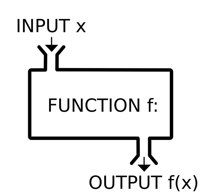
In mathematics, a function is just a ‘rule’ that relates inputs to outputs (with certain constraints).
Later you may have come across this formulation:
$$f(x) = 2x +3$$
Now the function has a name f() (not a particularly good one, however).
You probably recall that $x$ is called the argument of the function. So how do we translate this into R?
The crucial thing here is the R function() operator:
f <- function(x) {
  (2 * x)  + 3
}
We define the function using this function() operator, and also assign the function to a name (here f) using <-, just like assigning any other value to an object. This means that now f is a function object: just like you create vector objects, or lists, or data frame objects, when you assign them to names. Notice too that in RStudio they appear in the Global Environment in a special ‘Functions’ section, and clicking on them shows the code of the function. This means that if you have a large file with many functions defined, you don’t have to go back searching for the function definition in the code itself.
Terminology (gotta have it!)
x here is also called the argument to the function. In this case there is just one, there could be more.
The expression inside the curly braces: $(2 * x) + 3$, is called the body of the function.
Here is the basic template of any function in R:
name <- function(arg1, arg2...) {
  <body>
}
The arguments go inside (…). The body is the block of code you want to reuse, and it’s contained in curly brackets {…}.
Giving good names to functions can be tricky. You to don’t want to be too explicit, and you don’t want to be too terse (f() is too terse, btw). We’ll return to this below when we write fancier functions.
But now we want to actually use the function to compute an output: this is termed calling the function, by passing in a specific value. That specific value gets assigned to the argument inside the function.
Here is a trivial example, assigning the value $1$ to the argument:
f(1)
#> [1] 5
So after calling the function in this way x is instantiated to 1, and what is really happening is:
f <- function(1) {
  (2 * 1)  + 3
}
Easy-peasy.
But wait! if you simply call a function, its output (which you are probably interested in) just goes away. If you want to save the output of the function, to be used later, you need to assign the output to a variable:
my_output <- f(1)
my_output
#> [1] 5
This variable will now appear in the Values section of your Environment pane in RStudio, and can be reused in your subsequent code.
But wait! remember R data-structures? What if we pass in a vector as the argument?
f(c(1, 2, 3, 4, 5))
#> [1]  5  7  9 11 13
Woohoo! In R, the functions you write yourself are also automagically ‘vectorized’: vector in, vector out.
But wait! how about a list???
f(list(1, 2, 3, 4, 5))
#> Error in 2 * x: non-numeric argument to binary operator
Whoops! Looks like R is vectorized over vectors :). If we want to process our new function over a list we’ll have to do something more fancy, like a for-loop. We’ll see how to incorporate our own functions into for-loops, building on previous sessions, next week.
Breakout rooms, write your own functions
Exercise 1
Write a function from scratch that computes the square of a single input. Give it a sensible name, and run it on some test input numbers to make sure it works.
Make sure to look in the Functions pane of the RStudio Environment tab to check it is assigned correctly.
Is your function vectorized? Run it on a simple vector argument to check.
Hints (click here)
The relevant R exponentiation operator is `**`.
Solution (click here)
square <- function(x){
  x ** 2
}

square(2)
#> [1] 4
square(c(1, 2, 3, 4))
#> [1]  1  4  9 16
Exercise 2
The function in Exercise 1 has a single argument, the base, and raises it to the exponent 2.
Write a function with two arguments, which includes both a base and exponent and try it out.
Is your function vectorized? Run it on a simple base vector to check.
Bonus: is it vectorized on both the base and the exponent?
Exercise 3
R does not have a built-in function for calculating the coefficient of variation, aka the RSD (relative standard deviation). This is defined as the ratio of the standard deviation to the mean.
Create a function that computes this, and test it on a couple of vectors.
Hints (click here)
The relevant R built-in functions are
sd() and mean(). The function should have one argument, which is assumed to be a vector. Why write functions? (Spoiler alert, DRY…)
Copying your code is not good
The first motivation for writing a function is when you find yourself cut-and-pasting code blocks with slight alterations each time.
Say we have the following toy tidyverse data frame, where each column is a vector of 10 random numbers from a normal distribution, with mean = 0 and sd = 1 (the defaults for rnorm):
df <- tibble(
  a = rnorm(10),
  b = rnorm(10),
  c = rnorm(10),
  d = rnorm(10)
)

df
#> # A tibble: 10 × 4
#>          a       b       c      d
#>      <dbl>   <dbl>   <dbl>  <dbl>
#>  1 -1.88    0.727  -0.468   1.27
#>  2  0.0399 -0.789  -2.41    0.376
#>  3 -0.410   1.86    1.05   -0.618
#>  4 -0.266  -0.204  -0.715   0.279
#>  5  0.244  -0.0673  0.884  -0.340
#>  6  0.0645 -1.09    0.152  -0.840
#>  7  0.749  -0.494   0.681   0.341
#>  8 -1.35    0.208   0.0776  2.15
#>  9 -1.17    0.0883 -0.829  -0.174
#> 10  0.733   1.05    0.808   0.190
In previous Code Clubs we’ve seen how you can apply a built-in function like mean to each column using a for loop or lapply. But say we wanted to do something a bit fancier that is not part of core R. For example, we can normalize the values in a column so they range from 0 to 1 using the following code block:
(df$a - min(df$a)) / (max(df$a) - min(df$a))
#>  [1] 0.0000000 0.7297073 0.5582684 0.6132731 0.8073051 0.7390605 1.0000000
#>  [8] 0.1988908 0.2699569 0.9939179
This code is a literal translation of the mathematical formula for normalization:
$$z_{i} = \frac{x_{i} - min(x)}{max(x)-min(x)}$$
OK, so how can we do this for each column? Here is a first attempt:
df$a <- (df$a - min(df$a)) / (max(df$a) - min(df$a))
df$b <- (df$b - min(df$a)) / (max(df$b) - min(df$b))
df$c <- (df$c - min(df$c)) / (max(df$c) - min(df$c))
df$d <- (df$d - min(df$d)) / (max(df$d) - min(df$d))

df
#> # A tibble: 10 × 4
#>        a       b     c      d
#>    <dbl>   <dbl> <dbl>  <dbl>
#>  1 0      0.246  0.562 0.706
#>  2 0.730 -0.267  0     0.407
#>  3 0.558  0.630  1     0.0746
#>  4 0.613 -0.0691 0.490 0.375
#>  5 0.807 -0.0228 0.952 0.168
#>  6 0.739 -0.370  0.741 0
#>  7 1     -0.167  0.894 0.396
#>  8 0.199  0.0705 0.719 1
#>  9 0.270  0.0299 0.458 0.223
#> 10 0.994  0.356  0.930 0.345
This works, but it caused me mental anguish to type it out. Even with cut and paste! All those manual textual substitutions!! And manual data entry is prone to mistakes, especially repetitive tasks like this. And say you had 1,000 columns…
And it didn’t work!! Honestly, I swear that mistake was totally real: I didn’t notice it until I looked at the output. Can you spot the mistake?
It turns out R has a range function that returns the minimum and maximum of a vector, which somewhat simplifies the coding:
range(df$a)The result is a vector like c(-1.2129504, 2.1011248) (it varies run to run, since the columns values are random) which we can then index, and so we only do the min/max computation once for each column, instead of three times, so we get the following block of code for each column:
rng <- range(df$a)
(df$a - rng[1]) / (rng[2] - rng[1])
Does this help?
rng <- range(df$a)
df$a <- (df$a - rng[1]) / (rng[2] - rng[1])

rng <- range(df$b)
df$b <- (df$b - rng[1]) / (rng[2] - rng[1])

rng <- range(df$c)
df$c <- (df$c - rng[1]) / (rng[2] - rng[1])

rng <- range(df$d)
df$d <- (df$d - rng[1]) / (rng[2] - rng[1])
Still pretty horrible, and arguably worse since we add a line for each column.
How can we distill this into a function to avoid all that repetition?
Encapsulation of code in a function
The secret to function writing is abstracting the constant from the variable. (Using the range function does throw into sharper relief what is constant and what is varying at least.) The constant part is the body of the function: the template or boiler-plate you use over and over again. The variable parts are the arguments of the function.
Here’s what it looks like in this case:
normalize <- function(x) {
  rng <- range(x)
  (x - rng[1]) / (rng[2] - rng[1])
}
Pretty cool, right? Here normalize is the descriptive name we give the function.
In the current case the argument of our function is a column vector pulled from the data frame. But we can potentially use this function on any vector, so let’s not be too specific. The more generally you can write your function, the more useful it will be.
test_vec <- c(3, 7, pi, 8.657, 80)
normalize(test_vec)
#> [1] 0.000000000 0.051948052 0.001838866 0.073467532 1.000000000
A couple of things to note:
-
Including that extra line
rng <- range(x)is no longer a problem, since we just type it once. If you are typing things out over and over you might prefer brevity. When you write a function, you should prefer clarity. It’s good practice to break the the function down into logical steps, and name them properly. It’s much easier for others to ‘read’ your function, and much easier for you when you come back to it in a couple of years. This is the principle of making your code ‘self-annotated’. -
Functions should be simple, clear, and do one thing well. You create programs by combining simple functions in a modular manner.
Our original horrible code can now be rewritten as:
df$a <- normalize(df$a)
df$b <- normalize(df$b)
df$c <- normalize(df$c)
df$d <- normalize(df$d)
Which is an improvement, but the real power comes from the fact that we can use our new function in for loops and apply statements. We’ll see how to do that next week.
By writing our own functions, we’ve effectively extended what R can do. And this is all that packages are: libraries of new functions that extend the capabilities of base R. In fact, if there are functions you design for your particular subject area and find yourself using all the time, you can make your own package and load it, and all your favorite functions will be right there (but that’s for another day…)
Exercise 4: Functions are not just for arithmetic!
The fastq file format for DNA sequencing uses a letter/punctuation code for the quality of the base called at each position (the fourth line below) which is in one-to-one relationship to the bases in the second line:
@SIM:1:FCX:1:15:6329:1045 1:N:0:2
TCGCACTCAACGCCCTGCATATGACAAGACAGAATC
+
<>;##=><9=AAAAAAAAAA9#:<#<;<<<????#=
To translate a letter code into a numerical phred quality score we have to do two things: (i) translate the character to an integer using the ASCII code look up table (ii) subtract 33 from that value (!). (High scores are good).
For the first step, R has a built-in function that converts a character into an integer according to that table, for example:
utf8ToInt("!")
#> [1] 33
Write a function phred_score() that computes the phred score for any character. Check that it returns 0 for “!”.
Is this function vectorized? Apply your function to our example string:
<>;##=><9=AAAAAAAAAA9#:<#<;<<<????#=
to convert it to a vector of phred quality scores.
Hints (click here)
Remember when you pass the value to this function it has to be an R character string, which needs to be surrounded by quotes.
Solution (click here)
phred_score <- function(character){
  utf8ToInt(character) - 33
}

phred_score("!")
#> [1] 0
phred_score("<>;##=><9=AAAAAAAAAA9#:<#<;<<<????#=")
#>  [1] 27 29 26  2  2 28 29 27 24 28 32 32 32 32 32 32 32 32 32 32 24  2 25 27  2
#> [26] 27 26 27 27 27 30 30 30 30  2 28
Note: “!” is the first printing character in the ASCII table. The characters 0 through 32 were used historically to control the behavior of teleprinters: “the original ASCII specification included 33 non-printing control codes which originated with Teletype machines; most of these are now obsolete”. If the ASCII table started with “!” instead of NUL we wouldn’t need the correction of subtracting 33, and “!” would translate to 0.